4. Introduction
To meet increasingly stringent energy performance targets and challenges posed by distributed renewable energy generation on the electrical and thermal distribution grid, recent attention has been given to system-level integration, part-load operation and operational optimization of buildings. The intent is to design and operate a building or a neighborhood optimally as a performance-based, robust system. This requires taking into account system-level interactions between building storage, HVAC systems and electrical and thermal grid. Such a system-level analysis requires multi-physics simulation and optimization using coupled thermal, electrical and control models. Optimal operation also requires closing the gap between designed and actual performance through commissioning, energy monitoring and fault detection and diagnostics. All of these activities can benefit from using models that represent the design intent. These models can then be used to verify responses of installed equipment and control sequences, and to compute optimal control sequences in a Model Predictive Controller (MPC), the latter of which possibly requiring simplified models.
Furthermore, in the AEC domain the processes of designing, constructing and commissioning buildings and engergy systems are rapidly changing toward digitalization. Building Information Modeling (BIM) is an enabler as collaborative method and tool to consistently gather, manage and exchange building-related data on a digital basis over the entire life cycle of a facility. BIM is not a specific software, it is rather a method as part of, but not limited to, the integral design. A truly added value is expected for the near future when design and commissioning in the sense of computer aided facility management comes together. The above mentioned issues of commissioning, energy monitoring and fault detection and diagnostics can therefore highly benefit from a thorough digital planning when location and function of technical systems are together referenced in a digital model, when the as-built state is harmonized with and well documented in a model and when home and building automation becomes integrally linked with BIM.
This shift in focus will require an increased use of models throughout the building delivery stages and continuing into the operational phase. Consider, for example, the development and use of an HVAC system model:
- During design, a mechanical engineer will construct a model that represents the design intent, such as system layout, equipment selection, and control sequences. The basis of such a model could be from a BIM in the case of a building, or from a GIS in the case of a district.
- During construction, to reduce cost for implementation of the control sequence, and to ensure that the control intent is properly implemented, a control model could be used to generate code that can be uploaded to supervisory building automation systems, thereby executing the same sequence as was used during design [NW14].
- During commissioning, the design model will be used to verify proper installation.
- During operation, the model will be used for comparing actual with expected energy use [PWBH11], and for fault detection and diagnostics [BSG+14]. Furthermore, the model may be converted to a form that allows its use during operation as part of an MPC algorithm.
In addition to the focus on closing the performance gap between design and operation, another recent focus is on system integration. Here, the challenge lies in the co-design and operation of building dynamics, HVAC, thermal and electrical storage, renewable energy generation, and grid responsive control in order to maintain the power quality of the electrical grid. Commonly, to support system integration, models from different engineering domains need to be coupled during run-time. For example, for active facade control, it may be necessary to couple a ray-tracing tool such as Radiance with a building energy simulation tool to asses the impact of daylighting controls on reducing glare, energy, and peak cooling demand. Similarly, for building to electrical grid integration, building HVAC and domestic hot water control can be designed such that buildings present themselves as a flexible load to the electrical grid, which can increase the amount of renewable energy integrated into the grid. Such coupling of domain-specific models may be done within Modelica, an equation-based, object-oriented modeling language, or through tool coupling that involves co-simulation, a technique in which simulators exchange data as the simulation-time advances. See [Wet11a][BDCVR+12][BWN14][WBN16][CH15] for example applications.
For a larger discussion of functionalities that future building modeling tools will need to provide to address the needs for low energy building and community energy grid design and operation, we refer to [Wet11b] and [Cla15].
The aforementioned new foci give rise to new requirements for building simulation tools, including the following:
- Mechanical engineers should be able to design, assess the performance and verify the correctness of local and, in particular, supervisory control sequences in simulation. They should then use such a verified, non-ambiguous specification to communicate their design intent to the control provider. Moreover, the specification should be used during commissioning to verify that the control contractor implemented the design intent.
- Controls engineers should be able to extract subsystem models from models used during the building design in order to use them within building control systems for commissioning, model-based controls, fault detection and diagnostics.
- Urban planners and researchers should be able to combine models of buildings, electrical grids and controls in order to improve the design and operation of such systems to ensure low greenhouse gas emissions or costs, and high quality power delivery [BDCVR+12][WBN16][BWN14].
- Mechanical engineers should be able to convert design models to a form that allows the efficient and robust solution of optimal control problems as part of MPC [SOCP11]. Such models may then be combined with state estimation techniques that adapt the model to the actual building [BSG+14].
The first item requires modeling and simulation of actual control sequences, including proper handling of hybrid systems, i.e., systems in which the state evolves in time based on continuous time semantics that arises from physics, and discrete time and discrete event semantics that arises from digital control [Wet09][WZNP14]. This poses computing challenges for the deterministic synchronization of these domains [BGL+15]. The second item requires extraction of a subsystem model and exporting this model in a self-contained form that can readily be executed as part of a building automation system as shown in [NW14]. The third item requires models of different physical domains and models of control systems to be combined for a dynamic, multi-physics simulation that involves electrical systems, thermal systems, controls and possibly communication systems, which may evolve at vastly different time scales. The fourth item greatly benefits if model equations are accessible to perform model order reduction and to solve optimal control problems.
4.1. Comparison to State-of-the-art in Building Energy Modeling and Simulation
Today’s whole-building simulation programs formulate models using imperative programming languages. Imperative programming languages assign values to functions, declare the sequence of execution of these functions and change the state of the program, as is done for example in C/C++, Fortran or MATLAB/Simulink. In such programs, model equations are tightly intertwined with numerical solution methods, often by making the numerical solution procedure part of the actual model equations. This approach has its origin in the seventies when neither modular software approaches were implemented nor powerful computer algebra tools were available. These programs have been developed for the use case of building energy performance assessment to support building design and energy policy development. Other use cases such as control design and verification, model use in support of operation, and multi-physics dynamic analysis that combines building, HVAC, electrical and control models were not priorities, nor even considered [CLW+96]. However, the position paper of IBPSA shows that they recently gained importance [Cla15].
Tight coupling of numerical solution methods with model equations and input/output routines makes it difficult to extend these programs to support new use cases. The reason is that this coupling imposes rules that determine for example where inputs to functions that compute HVAC, building or control equipment are received from the internal data structure of the program, when these inputs are updated, when these functions are evaluated to produce new output, and what output values may be lagged in time to avoid algebraic loops. Such rules have made it increasingly difficult for developers to add new functionalities to software without inadvertently introducing an error in other parts of the program. They also make it difficult for users to understand how component models interact with other parts of the system model, in particular their interaction with, and assumptions of, control sequences. Furthermore, they also have shown to make it difficult to use such tools for optimization [WW04].
The tight coupling of numerical solution methods with model equations also makes it difficult to efficiently simulate models for the various use cases. Numerical methods in today’s building energy simulation programs are tailored to the use case of energy analysis during design. However, other use cases, such as controls design and verification, coupled modeling of thermal and electrical systems, and model use during operation require different numerical methods. To see why different numerical methods are required, consider these applications:
- Stiff systems: The simulation of feedback control with time constants of seconds coupled to building energy models with time constants of hours leads to stiff ordinary differential equations. Their efficient numerical solution requires implicit solvers [HW96].
- Non-stiff systems: In EnergyPlus [CLP+99] and in many TRNSYS [KDB76] component models, the dynamics of HVAC equipment and controllers, which is fast compared to the dynamics of the building heat transfer, is generally approximated using steady-state models. Hence, the resulting system model is not stiff as the only dynamics is from the building model. In this situation, explicit time integration algorithms are generally more efficient. Such an approximation of the fast dynamics can also be done with dynamic Modelica HVAC models, see [JWH15].
- Hybrid systems: Hybrid systems require proper simulation of coupled continuous time, discrete time and discrete event dynamics. This in turn requires solution methods with variable time steps and event handling. For example, when a temperature sensor crosses a setpoint or a battery reaches its state of charge, a state event takes place that may switch a controller, necessitating solving for the time instant when the switch happens and reducing accordingly the integration time step. Standard ordinary differential equation solvers require an iteration in time to solve for the time instant of the event, and reinitializing integrators after the event, which both are computationally expensive. A new class of ordinary differential equation solvers called Quantized State System (QSS) integration [ZL98][KJ01][CK06][Kof03][MBKC13] are promising for the efficient simulation of such systems as they do not require iteration for state event detection. However, their efficient use requires knowledge of the dependency graph of the state equations, which generally is not available in legacy building simulators, but readily available in equation-based languages.
It follows from this discussion that for models to be applicable to a wide range of applications, it should be possible to use them with different numerical solvers. Therefore, models for building energy systems and their numerical solution methods should be separated where possible. Exceptions are equations for which special tailored solution methods and parallel programming patterns allow humans to better exploit the structure of the equations than is currently supported by code generators, often arising from partial differential equations or from light distributions. Examples include solvers for computational fluid dynamics, heat transfer in borehole heat exchangers [PH14], and ray-tracing for daylighting. Work, however, is ongoing to remedy this situation [Cas15][SWF+15][BBCK15].
4.2. New Technologies for Building Energy Modeling and Simulation
This section describes new technologies which can be applied to building energy modeling in support of the different use cases.
4.2.1. Equation-based Modeling
As explained above, the use of imperative programming languages limits the applicability and extensibility of models. Furthermore, in building simulation programs, numerical solution algorithms are often tightly integrated into the models and thereby can mandate the use of supervisory control logic that is far removed from how control sequences are implemented in reality. For example, in EnergyPlus, a cooling coil may request from the supervisory control a certain air mass flow rate in order to meet the load computed in the predictor step of the thermal zone heat balance. In actuality, the air mass flow rate would be determined by the position of dampers in combination with the speed of a supply fan, each of which could be controlled by zone temperature and duct static pressure feedback controllers.
A key difference between imperative programming languages and equation-based languages is that the latter do not require a specification of the sequence of computer assignments required to simulate a model. Rather, a model developer can specify the mathematical equations, package them into graphically represented components and store them in a hierarchical library. A model user then assembles these components in a schematic editor to form a system model. A simulation environment analyses these equations, optimally rearranges them using computer algebra, translates them to executable code, typically C, and links them with numerical solvers.
Specifically, the translation of equations to executable code involves determining which variables can be replaced by so-called alias variables, for example, in the case of a mass flow rate that may be the same for all components that are used to compose an air handler unit. It also involves reducing the dimension of coupled linear and nonlinear system of equations through symbolic inverting equations and through Block Lower Triangularization and Tearing [CK06][EO94], which often significantly reduces the dimension of the coupled systems of equations. See also Section 5.3.4. Furthermore, during translation, zero-crossing functions are generated, for example, to indicate when a thermostat crosses a set-point, and high-order differential algebraic systems of equations are reduced to index 1 [MS93]: Some Modelica translators also generate code for specific solvers. The benefit of this has been demonstrated by Fernandez and Kofman who showed for QSS methods more than an order of magnitude simulation speed improvements when code is generated in a form that is specifically designed for the QSS methods [FK14], as opposes to using QSS methods with a conventional discrete event simulation solver. Symbolic manipulations also allow to partition the model automatically for parallel computing [EMO14].
Loosely speaking, while simulation models implemented using imperative programming languages require numerical solvers to select numerical inputs and compare the function values for these inputs to infer what equations they solve, equation-based modeling languages such as Modelica allow for the understand of equation structure, and making use of this understanding to generate efficient code for computation. Examples of structures include which variables are connected to each other through algebraic constraints or differential equations, which equations can be differentiated, which equations can be inverted, and which equations trigger an event that can instantly change a control signal. For a more detailed discussion, see [Elm78], [CK06], [EO94] and [EOC95]. To make these technologies accessible to a wide range of users in building simulation, research and development is required and ongoing to advance translators and solvers to better handle large models [Wet09][Zim13][WZNP14][JWH15][Cas15][SWF+15][BBCK15].
A promising aspect of Modelica is that it is an open-source language that is supported internationally by various industries. As these industry sectors use the same modeling language, modeling environments, simulation and optimization code generators and solvers, the investement in these technologies can be shared. Consequently, large international projects that further advance Modelica have been conducted, such as
- MODELISAR (https://itea3.org/project/modelisar.html, 29 partners, Euro 26.6M, 2008-2011) which initiated the FMI standard,
- EUROSYSLIB (http://www.eurosyslib.com/, 19 partners, Euro 16M, 2007-2010) which developed Modelica libraries for embedded system modeling and simulation, and
- MODRIO (https://www.modelica.org/external-projects/modrio, Euro 21M, 2012-2015) which extended Modelica and FMI to support property/requirement modelling, state estimation, multi-mode modelling, e.g., systems with multiple operating modes and varying number of states, and nonlinear model predictive control.
4.2.2. Co-Simulation and Model Exchange
In 2008, a European project called MODELISAR started with the objective to facilitate interoperability between simulation models and simulation tools through a standardized application programming interface (API). This project resulted in the Functional Mockup Interface (FMI) standard, which is a tool-independent, open-source standard which supports exporting, exchanging and importing simulation models or simulation tools [MC14].
A simulation model or a complete simulator that is exported in the format specified by the FMI standard is called a Functional Mockup Unit (FMU). The FMI standard defines a set of C-functions (FMI functions) to interact with the model or the simulator. It also defines an xml schema that is used to declare properties of the exported model or simulator. In addition, it standardizes how to package as a zip file the xml file, the C-functions, possibly as compiled binaries, and resources required by the model or simulator, such as files with weather data.
The FMI standard distinguishes between model-exchange and co-simulation. In FMI for model-exchange, a system of differential, algebraic and discrete-time equations can be exported, and the host simulator that executes the FMU needs to provide an algorithm that integrates the equations in time. In contrast, in FMI for co-simulation, the host simulator requests the FMU to integrate its equations in time. See for example [BBG+13] for such an algorithm.
Version 2.0 of FMI standard was released in 2014, and it adds features that will facilitate the use of FMU models to support the design and operation of buildings. Some of the important features are as follows:
| Saving and restoring the state: | |
|---|---|
The complete FMU state can be saved, restored, and serialized to a byte vector. As a result, a simulation can be restarted from a saved FMU state. This is a very important feature for model-based fault detection as the one in [BSG+14] or model predictive controls applications as both of them require state initialization. |
|
| Input and state dependencies: | |
In the xml file, it can be declared which state variables and which output variables have a direct dependency on the input variables, and which output variables have a direct dependency on the state variables. This allows
The information about dependency also opens the door to the implementation of efficient asynchronuous numerical time integration algorithms such as QSS. Furthermore, for FMUs that are connected to form a cyclic graph, the dependency information of outputs on inputs is required for the deterministic execution [BBG+13], and the detection of algebraic loops. Once those algebraic loops are detected, nonlinear equation solvers such as a Newton-Raphson solver can be used to solve them. The following example, which is borrowed from [BBG+13], illustrates why exposing such dependencies is important. Consider the FMU that comprises the system shown in Fig. 4.1. If this FMU is imported in a simulator and \(y_1\) is connected to \(u\), possibly using an algebraic function \(f \colon \Re \to \Re\), then a master algorithm can output the state \(y_1\), assign \(u = f(y_1)\), output \(y_2 = -5 \, u\) and integrate the state. If however \(u\) were connected to \(f(y_2)\) rather than \(f(y_1)\), then a master algorithm can output \(y_1\), next it needs to solve \(u = f(y_2) = -5 \, f(u)\), in general using numerical iterations, and then it can integrate the state. This illustrates that input-output dependency is important as it allows a simulator to detect whether cyclic graphs, formed by connecting inputs and outputs among FMUs, lead to an algebraic system of equations that may require an iterative solution. See [BBG+13] for a more detailed discussion. 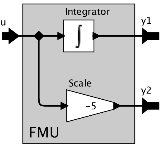
Fig. 4.1 FMU for which output \(y_1\) does not have a direct dependency on input \(u\) but output \(y_2\) does. |
|
| Directional derivatives: | |
Directional derivatives can be computed for derivatives of continuous-time states and for outputs. This is useful when connecting FMUs and the partial derivatives of the connected FMU shall be computed, for example by a stiff ordinary differential equation solver, an algebraic loop solver, an extended Kalman filter, or for model linearization. If the exported FMU performs this computation analytically, then all numerical algorithms based on these partial derivatives are more efficient and more reliable [MC14]. Directional derivatives are also required by second-order QSS algorithms [Kof03]. This is illustrated with the following example. Consider an FMU which implements \(dx(t)/dt = f(x,u,t)\) for some differentiable function \(f \colon \Re \times \Re \times \Re \to \Re\). If the FMU provides directional derivatives, then the second time derivative can be computed exactly because
\[\frac{df(x,u,t)}{dt}=\frac{\partial f(x,u,t)}{\partial x} \frac{dx(t)}{dt} +
\frac{\partial f(x,u,t)}{\partial u} \frac{du(t)}{dt},\]
where \({\partial f(x,u,t)}/{\partial x}\) and \({\partial f(x,u,t)}/{\partial u}\) are the directional derivatives with respect to state and input, which are provided by the FMU. |
|
In summary, there are various benefits in using equation-based languages, such as Modelica, for system simulation. First, they allow for sufficient semantics for a code generator to identify the state variables in a model, which supports saving and restoring states for initializing simulations. Second, they allow for the discovery of input-output and input-state dependencies, which supports master algorithm development. Lastly, they allow for automatic differentiation of model equations, which supports in providing directional derivatives to solvers. While these pieces of information could in principle also be specified by a model developer in models that are written using imperative languages, the size of models typically encountered in building simulation would make such a manual declaration a tedious, expensive and error-prone proposition.
The relevance of these properties for the building simulation community has been illustrated in the following examples. Broman et al. [BBG+13] developed a master algorithm for the deterministic composition of FMUs for co-simulation, which is only possible if input/output dependencies are provided for FMUs that are connected in a cyclic graph. Wetter et al. [WNL+15] simulated a building with radiant heating system using a collection of FMUs for model exchange that are asynchronously integrated in time using QSS methods. The input-state dependencies were required to determine which state variables need to be updated. Bonvini et al. [BWS14] have developed and applied an FMU-based state and parameter estimator that has been used as part of a fault detection algorithm which is capable of identifying faults in a valve. This algorithm required saving and restoring states.
The capabilities of FMI and the aforementioned use cases indicate its applicability to support building simulation for design and operation. At the time of writing, there are more than 70 tools which support import or export of simulation models or tools as FMUs. This indicates the adoption of the standard and its relevance for the building simulation community.
4.2.3. Optimization
Equation-based modeling languages allow code generators to convert model equations to a form that is well suited to solve large scale nonlinear optimization problems [AAG+10]. This section describes a state of the art method that converts an infinite dimensional optimal control problem into a finite dimensional approximation that standard nonlinear programming (NLP) solvers can solve. Equation-based modeling languages allow automating this conversion.
Equation-based modeling languages allow to describe systems of differential algebraic equations (DAE) in the general form
where \(F(\cdot, \cdot, \cdot, \cdot, \cdot, \cdot)\) describes the time rate of change, \(Y(\cdot, \cdot, \cdot, \cdot, \cdot)\) are algebraic constraints, \(F_0(\cdot, \cdot, \cdot, \cdot, \cdot)\) implicitly defines initial conditions, \(t \in [t_0, \, t_f]\) is time for some initial and final time \(t_0\) and \(t_f\), \(x \colon \Re \to \mathbb{R}^{n_x}\) is the state vector, \(u \colon \Re \to \mathbb{R}^{n_u}\) is the control function, \(y \colon \Re \to \mathbb{R}^{n_y}\) is the vector of algebraic variables, and \(\Theta \in \mathbb{R}^p\) is the vector of parameters. Such a DAE system can be used to model a building, its HVAC systems and controllers. Necessary and sufficient conditions for existence, uniqueness and differentiability of a solution to (1) can be found in [Wet05].
Once the model is available, we can add constraints and a cost function to define an optimal control problem that minimizes energy consumption or cost. An example optimal control problem for (1) is
for all \(t \in [t_0, \, t_f]\), where \(f(\cdot, \cdot, \cdot, \cdot)\) is the cost function and \(\mathcal U\) is the set of admissible control functions. The solution to (2) is the optimal control function and the optimal design parameter that minimizes \(f(\cdot, \cdot, \cdot, \cdot)\) while satisfying the system dynamics \(F(\cdot, \cdot, \cdot, \cdot, \cdot, \cdot) = 0\), and \(Y(\cdot, \cdot, \cdot, \cdot, \cdot) = 0\), the initial conditions \(F_0(\cdot, \cdot, \cdot, \cdot, \cdot) = 0\) and the constraints \(H(\cdot, \cdot, \cdot, \cdot, \cdot, \cdot) = 0\) and \(G(\cdot, \cdot, \cdot, \cdot, \cdot, \cdot) \leq 0\). For generality, we assume (2) to be nonlinear and twice continuously differentiable [Pol97].
The problem (2) is infinite dimensional because its solution is a functional that has to be valid for all \(t \in [t_0, \, t_f]\). Directly solving an infinite dimensional optimal control problem for a general nonlinear system is not possible and it therefore needs to be converted into a finite dimensional approximation [Pol97]. Biegler [Bie10] presents multiple methods for such a conversion into the form
where \(z\) is the finite dimensional optimization variable, \(z^{l}\) and \(z^{u}\) are the lower and upper bounds, \(c(\cdot)\) is the cost function, and \(g(\cdot)\) and \(h(\cdot)\) are the equality and inequality constraints.
Among the available techniques, we describe direct collocation methods because they are well suited for equation-based modeling languages [AAG+10]. Direct collocation methods use polynomials to approximate the trajectories of the variables of a DAE system. The polynomials are defined on a finite number of support points that are called collocation points. By optimizing these finite number of control points, they convert the infinite to a finite dimensional optimization problem, which can be solved by a NLP solver such as IPOPT [WB06].
The method starts by dividing the time horizon \([t_0, \, t_f]\) into \(n_e\) elements, each element containing the same number of collocation points \(n_c\). For example, the JModelica software [AGT09] uses the Radau collocation method to place these points. The Radau collocation method places a collocation point at the start and end of each element to ensure continuity of the state trajectories, and places the others to maximize accuracy. In each element, time is normalized as \(\tilde{t}_i(\tau) = t_{i-1} + h_i \, (t_f - t_0) \, \tau\), for \(\tau \in [0, \, 1]\) and \(i \in \{1, \, \ldots, \, n_e\}\), where \(t_i\) is the time at the end of element \(i\), \(\tau \in [0, \, 1]\) is the normalized time within the element, and \(h_i\) is the length of element \(i\). The time dependent variables \(\dot{x}(\cdot)\), \(x(\cdot)\), \(u(\cdot)\), and \(y(\cdot)\) are approximated using collocation polynomials in each element. The collocation polynomials use the Lagrange basis polynomials, and they use the collocation points as the interpolation points. The collocation polynomials are
where \(x_{i,k}\), \(u_{i,k}\), and \(y_{i,k}\) are the values of the variable \(x(\cdot)\), \(u(\cdot)\) and \(y(\cdot)\) at the collocation point \(k\) in element \(i\), \(l_k(\cdot)\) is the Lagrange basis polynomial and \(\tilde{l}_k(\cdot)\) is the Lagrange basis polynomial that includes the first point to ensure continuity of the state variables. The Lagrange bases are, with \(i \in \{1, \, \ldots, \, n_e\}\),
As \(\tau\) is normalized, the basis polynomials are the same for all elements. The polynomial approximation of the derivative \(\dot{x}_i(\cdot)\) in (3) is
The collocation method defines the approximations (3) and (5) of the variables in (2). Equation-based modeling languages allow accessing the model equations, thereby allowing to automatically generate the finite dimensional approximations defined by the collocation methods.
JModelica employs a collocation method to transcribe the problem (2) into an NLP problem. A local optimum to the finite dimensional approximation of (2) will be found by solving the first-order Karush-Kuhn-Tucker (KKT) conditions, using iterative techniques based on Newton’s method. This requires first- and second-order derivatives of the cost and constraint functions with respect to the NLP variables. JModelica uses CasADi [And13], a software for automatic differentiation that is tailored for dynamic optimization. Equation-based modeling languages allow for automatically providing the information required by CasADi to build a symbolic representation of the optimization problem. Using the symbolic representation of the NLP problem, CasADi can efficiently compute the required derivatives and exploit the sparsity pattern of the problem. NLP solvers such as IPOPT are then used to find a piecewise polynomial approximation of the solution to the original problem (2). The number of variables in the approximated problem is \(n_z = (1 + n_e \, n_c) (2n_x + n_u + n_y) + (n_e - 1) n_x + n_p + 2\). For a more detailed overview see [MA12].
In summary, equation-based modeling languages provide three main advantages for optimization: First, they support the automatic conversion of simulation models into optimization problems, reducing engineering costs and time. Second, they can provide analytic expressions for gradients to be used by NLP solvers. Third, they allow for automatic generation of the finite dimensional approximations defined by the collocation methods.
Section 9.4.3 shows how this improves computing performance relative to simulation-based optimization.
4.2.4. Building Information Modeling
Building Information Modeling (BIM) provides methods, interfaces and tools for the integral design, construction, commissioning and operation of buildings. It is furthermore an enabler for quality assurance and digital documentation of the as-built state and to manage other building life cycle-relevant data [ETSL11]. Managing projects with BIM promises major improvements in the adherence of schedules, in transparency and in cost control [VIB15], if a BIM project is properly set-up and run. Digital planning methods are a key element for the design, commissioning and operation of energy efficient buildings, energy systems and city quarters at the interface between building envelope, building systems, distribution network, automation and control.
BIM-related processes may comprise the coordination of different models of the architecture, engineering and construction (AEC) domains, for example involving advanced rule-based model checker software. On the other hand, BIM may be applied for domain-specific planning tasks within the building services and HVAC domains. Thereby, a CAD model can serve as basis for layout and dimensioning, for engineering and code compliance testing, clash detection, or static and dynamic heat and cooling load calculations, for example.
Today, powerful CAD tools exist for the AEC domain which can be used for design and construction of HVAC systems. Some of these tools provide built-in and proprietary solutions for static or dynamic calculations building on their internal core and data model.
However,
- the lack of open-source solutions to support a tool-chain for BPS model transformation from BIM using open data formats such as the Industry Foundation Classes (IFC) makes it difficult to make BIM models available for BPS.
- Other BPS-related data formats such as gbXML are mainly restricted to geometrical issues and disregard parameter which are relevant for describing properties of HVAC components or control sequences.
- Current BIM formats lack the objects and semantics needed to express control logic, e.g., the algorithms that turn measured signals and set-points into actuator signals.
- Defining and generating an integrated building performance simulation model representing the building geometry and topology as well as its energy systems can be a cumbersome and error-prone procedure [BMOD+11].
- Furthermore, a CAD or BIM model cannot be readily transformed into an object-oriented simulation model, as the structure of both prevailing modeling worlds differ significantly [vTR06]. Models may be hampered by diverse inconsistencies due to modeling failures or inconsistencies or simply due to conceptual differences between the AEC domains and their modeling hierarchy, especially from a geometrical and topological point of view concerning the issue of space boundaries [BK07].
- The representation of CAD objects and its parameters in the HVAC domain itself differs from the representation which is needed in an object-oriented BPS model such as Modelica. In BIM, objects may not be properly linked with each other, or the way, how these objects are mutually connected may not be eligible for a model transformation into Modelica code which assumes objects are connected as in the real world through fluid ports.
These constraints often make it necessary to manually re-generate a BPS model from scratch instead of converting an existing CAD model to a BPS-like representation.
4.2.5. Overview of the Following Chapters
The next chapters describe the activities conducted in Annex 60.
Activities 1.1 to 1.4 were focused on the development of technologies for modeling, co-simulation, BIM to Modelica translations and workflow automation developed in Subtask 1. Activity 1.1, described in Section 5, gives an overview about Modelica and the Modelica Annex 60 library developed in this project. Activity 1.2, described in Section 6, introduces co-simulation using the FMI standard and presents FMI compliant tools and FMI capabilities of building energy simulators. Activity 1.3, described in Section 7, introduces BIM and presents an open framework for Modelica code generation from BIM. Lastly, Activity 1.4, described in Section 8, presents tools and examples for workflow automation in building and district energy simulation.
Activities 2.1 to 2.3 were focused on the validation and demonstration of the technologies developed in Subtask 2. Activity 2.1, described in Section 9, presents case studies that involve Modelica-based simulation and optimization at the building scale. Activity 2.2, described in Section 10, provides an overview about district energy systems. It then introduces first efforts to develop a validation test procedure for district energy system simulations called DESTEST, and it closes with examples of district energy simulation using mono-simulation and co-simulation. Activity 2.3, described in Section 11, describes use of Modelica and FMI for Fault Detection and Diagnostics, for Model Predictive Control, and for Hardware-in-the-Loop experimentation.
Concluding remarks can be found in Section 13, and a glossary for technical terms can be found in Section 14.