7. Activity 1.3: BPS Code Generation from Building Information Models
7.1. Introduction
Activity 1.3 of the Annex 60 is dedicated to the complex issue of transforming a digital model of a building and its energy systems into Modelica code that can be readily used for advanced building performance simulation (BPS). It is the conceptual idea and vision of this activity to thoroughly address the prevailing tedious, cumbersome and error-prone process of manual data conversion and model generation and to provide a methodology for automatically, or at least semi-automatically, transforming a digital model into an object-oriented acausal model.
The transformation is hampered by several constrains such as
- models contain inconsistencies and modeling errors and are typically not built by a person skilled in energy performance simulation,
- models originate in the design process from other domains such as the architecture or structural domain,
- objects and parameters in a CAD model significantly differ from the representation needed in Modelica,
- input models are lacking information relevant for BPS,
- a conversion process needs to support multiple Modelica libraries with different model topologies and varying syntax at the same time,
- the object-oriented data schema of the digital building model is continuously updated and subject to changes which need to be dynamically reflected by the tool.
Consequently, several complex requirements form the specification of a software framework that is capable to deal with these constraints. Furthermore, a flexible methodology is required to take expert knowledge into account when it comes to object and parameter mapping. The software framework shall provide interfaces to Open BIM data formats such as the Industry Foundation Classes (IFC). And, as well, the framework must be modularly structured in order to allow for further and distributed developments on an open source basis by an international community. Its structure shall allow to maintain the framework or even most parts of it in due time.
In order to carefully consider these settings, the activity followed the following approach:
- As BIM data format, the Annex supports the Open BIM format Industry Foundation Classes (IFC). Before processing BIM models, these models are checked for integrity concerning two aspects. First, the geometric consistency is accounted for by an advanced model checking process which includes the definition of space boundaries. Secondly, the HVAC model is checked by another model checking toolbox developed in this project.
- Models are then transformed into an intermediate data format called SimXML. Therefore, a flexible module for schema parsing was developed. Relevant data which are missing in the BIM can be added to the SimXML data model.
- In order to manage these SimXML data, a dynamic schema parser was developed in C++. This offers the flexibility to dynamically account for changes and updates of the SimXML schema (and, thus, for changes of the IFC data model as well). An application programming interface (API) between C++ and Python was implemented to efficiently interact with the data model.
- An object and parameter mapping mechanism as well as respective mapping rules were developed in order to formulate engineering knowledge in a rule-based methodology. These rules are processed by the framework.
- An IFC model view definition (MVD) was developed in order to specify the subset of IFC data relevant to BPS.
- In order to dynamically support multiple Modelica libraries at the same time, a template-based approach was selected as solution and implemented in Python.
- All transformation tools and methods are provided as open source framework for further developments in the community. Researchers are invited to collaborate and to further extend the framework.
The following sections briefly introduce what BIM is, explain the BIM data import process and detail the developed open Annex 60 framework for Modelica code generation from BIM. At the end of the chapter, the use cases applied for testing and development are introduced as well. It shall be noted at this point, that the activity followed a bottom-up approach which was based on these use cases. Therefore, the framework is currently limited to support these cases. As the activity focused on a subset of IFC data, on the other hand, with the resources on hand it was possible to finalize the overall framework as such in the Annex and to provide a modular framework for further development and dissemination.
7.2. Building Information Modeling (BIM)
This subchapter starts by introducing the term BIM and by explaining the changes required when BIM is used in a project. For the evaluation of the developed model transformation and BPS code generation concept and toolchain the use cases and case study are described next. The authors detail current state-of-the-art toolboxes and tools that are relevant for our prototype development. Finally, in this subchapter we summary relevant standards and agreements that are needed for development of BIM based data exchange.
7.2.1. What is BIM?
The acronym BIM stands for Building Information Model or Modeling. It involves buildings and building designs, information about given buildings and/or designs, and to how that information is modeled. Searching the term BIM on the web one will find many industry definitions such as: BIM and Sustainability, Green BIM, 4D BIM, BIM and the Bottom Line, BIM for Risk Management, BIM BOP, BIM CON!FAB, BIM Symposia, BIM Consulting, BIM Surveys, and many more. It seems that anybody who is asked to define BIM has their own definition which reflects their own needs, expectations and uses of BIM.
According to Bazjanac [Baz04], the BIM acronym can have two meanings: noun or verb. The science definition of BIM-the-noun is straight forward:
A Building Information Model (BIM) is an instance of a populated data model of buildings that contains multi-disciplinary data specific to a particular building which they describe unambiguously.
The science definition of BIM-the-verb is even simpler:
Building Information Modeling (BIM) is the act or process of creating a Building Information Model (BIM-the-noun).
Charles Eastman and colleagues offer a more elaborate and practical working definition of BIM for the buildings industry [ETSL11]:
BIM is a modeling technology and associated set of processes to produce, communicate, and analyze building models characterized by
- Building components that are represented with intelligent digital representations and can be associated with computable attributes and parametric rules.
- Components that include data that describe how they behave.
- Consistent and non-redundant data.
- Coordinated data such that all views of the model are represented in a coordinated way.
Similarly, definitions of BIM by buildingSMART International [bSI15a], the U.S. National Institute for Building Sciences [NIB16] and the U.S. National BIM Standard Project [NIB13] are in full concordance with this definition.
Eastman and colleagues also define what causes a data agglomeration not to be a BIM, disqualifying building “models” which some industry members call BIM:
- Building models that contain 3D data only and no object attributes.
- Building models with no support of behavior (i.e. models that do not utilize parametric intelligence).
- Building models that are composed of multiple 2D CAD reference files that must be combined to define the building.
- Building models that allow changes in one view that are not automatically reflected in other views.
Accordingly, a Building Information Collection (BIC) is also not a BIM. A BIC is characterized by an ad-hoc database to which information is supplied as a participant recognizes the need for it, with no systematically rules for database creation. As a result, the database is used indiscriminately from one building to another, and when viewing a datum in the database one cannot be confident what the datum actually represents without examining why and how the datum has been entered in the database.
In order to create a proper BIM, three conditions must be satisfied: (1) valid building data must be available and verifiable; (2) a specific data model of buildings must be used in the instantiation of data; and (3) software capable of properly populating the data model must be available and used in all instances of entering data in the data model. BIM data used in this research project are valid and verifiable for the purposes of the project. The most common data model format used with BIM is Industry Foundation Classes (IFC). The latest IFC version 4 Addendum 2 (IFC4 Add 2) [bSI15b] release is the data model used as basis for the BIM applications to share information across multiples software. All software used to populate the BIM is directly or indirectly IFC compatible.
IFC is fully object-oriented and is fully extensible. It is absolutely “neutral” (i.e. does not favor any software environment, platform, market, endeavor or suite of tools). IFC is also the only life cycle model of buildings that is an “open” International Standard Organization (ISO) Standard (no. 16739), and can be used free of charge.
The main purpose of the IFC data model is the enabling and support of software interoperability in the buildings industry. Software interoperability – essential to collaborative design – is the common name of technologies that allow software to communicate to one another and seamlessly share and exchange data. Some advantages of interoperability are detailed below:
- Allows automatic and flawless exchange of relevant common project data between one software application and another.
- Supports automatic data conversion between software that use partially overlapping data.
- Offers consistency management of the various ways that are used to model a building.
- Provides the tracking and management of information consistent with best practices required for security, provenance, etc. in support of contractual and legal frameworks.
Interoperable applications enable the work of multiple disciplines with varied expertise, and automatically translate data to support the different data structuring and viewing needs for different decision-making industry domains.
Any complete BIM of a sizeable commercial building will contain much more data than any single software application can read and manipulate. The main reason for that is not necessarily the size of the building – it is the multi-disciplinary nature of the data in a complete BIM. In most cases only discipline software can populate the BIM with all relevant discipline data, and only discipline software can read such data. To avoid having to deal with data in the BIM that are irrelevant to the discipline, relevant data are grouped and agglomerated in a “view” of the particular BIM [Hie06] and such views are defined as Model View Definitions (MVD).
Data included in Model View Definitions (MVD) are subsets of the IFC data model. The subsets specify all discipline (or project type) definitions in the IFC data model that need to be shared or exchanged among multiple software applications in support of work of a given discipline, project type or any other given purpose. bSI certifies software applications’ compliance with a given MVD if the application can demonstrate that all data exchange requirements of the given MVD (object/attribute/relationship sets, as well as their form and format) have been implemented by the application.
The BIM Collaboration Format (BCF) is an open XML file format that supports workflow communication and messaging among different software applications engaged in BIM processes [bSI14]. It boosts collaboration in BIM workflows by exchanging only the lean machine-readable BCF-topics with attached BIM-snippets (and not the entire BIM) among participating applications. The RESTful API enables seamless automated exchanges of BCF-topics among software that has implemented this Application Protocol Interface [bSI15c].
7.2.2. Changes Within the Planning/Design Process
The adoption of BIM (as a verb) constitutes a paradigm shift in the Architectural, Engineering, Construction and Facilities Management (AEC/FM) industry. BIM based collaboration is a different way of working as opposed to complementing the traditional 3D CAD approach. The key difference is the opportunity for collaboration over the entire building life-cycle: from conception to design, construction and operation and up to the final demolition. The deployment of BIM in construction can make the industry more efficient, effective, flexible and innovative [THN13]. However, the use and adoption of a new technology begins with a series of decisions that ends in appropriate and effective use of such technologies.
In some countries such as USA, UK, Norway, Finland, Denmark, Singapore and South Korea the use of BIM in projects is obligatory. Despite the industry’s awareness of the potential of BIM, construction organizations are yet to use it effectively. Fig. 7.1 shows that BIM is leading a change in resource allocation and associated costs from the later to the earlier stages of the project. By comparing the traditional 3D CAD approach with BIM, BIM is considered more efficient and less-time consuming, therefore less costly.
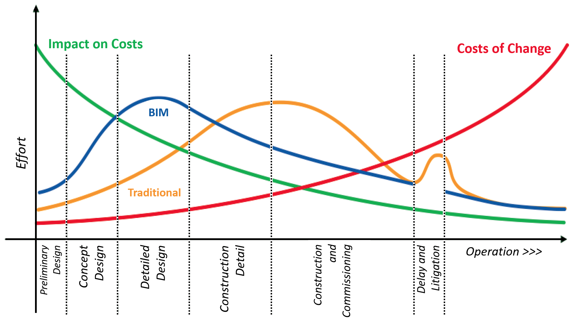
Fig. 7.1 Comparison between BIM-based workflow and traditional workflow (Adapted from [EHLP13]).
The use of BIM concentrates stakeholder collaboration throughout the entire building life-cycle. In doing so it provides a central repository of information that can be accessed by any stakeholder, when needed, in order to make the best and most effective use of available information. The major benefits from this approach are design consistency and visualization, cost estimates, clash detection and implementation of lean construction [VSS14]. This digital transformation cannot happen unless there are appropriately skilled personnel to support BIM implementation.
7.2.2.1. Roles and Responsibilities in the BIM-Based Process
It is expected that the demand for BIM will required new organizational structure and changes of responsibilities within defined roles. [GT14] on their study reviewed over 300 jobs description to determine responsibilities and skills required in BIM related roles. They identified three core roles: BIM Manager, BIM Coordinator and BIM Modeler. Others researches also mentioned different terminologies for these roles but with the same responsibilities of management, coordination and modeling [BS10][PH13][SML13].
A BIM Manager is a person familiar with the building and design process from start to finish. This role does not require a domain identifier as this is an overarching role within the organization covering all aspects such as collaborative information management, standards management and process planning. This person can work directly with BIM Coordinators and BIM Modelers and with management designing processes. The BIM Coordinator is the person responsible for facilitating the transition into BIM based work practices and subsequently enhance the performance of BIM based activities. This person’s key role is to help with the model and other BIM related issues. Lastly the BIM Modeler requires a domain identifier and skillset in their respective. This person focuses on a specific performance aspect of the project. Therefore, the success of a project depends on meaningful integration of the roles involved, through an efficient and sustainable use of BIM.
7.2.2.2. Agreements in the BIM Process
Different national and international BIM guidelines and standards are available today to help organizations to implement BIM in their processes [EHLP13][AECUKC15][BIMGW12]. The benefits of using BIM depends on the manner in which information will be created, maintained and shared within project stakeholders. People involved in the BIM project are expected to have the ability to produce, manage and share any information required in a standard format. According to Egger [EHLP13], the success of a project in the building industry depends on four factors: people, processes, guidelines and technology (Fig. 7.2). With the exception of technologies that are well established in the construction industry, the remaining three factors present problems that need to be overcome, especially the lack of professional training and guidelines.
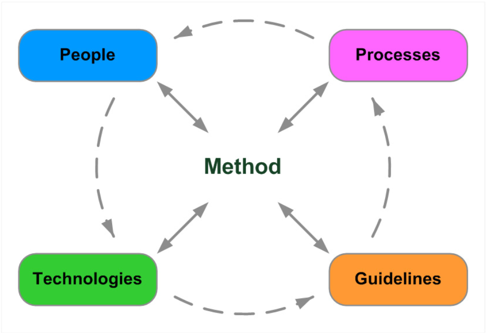
Fig. 7.2 Main factors of influence on the use of BIM method [EHLP13].
Within BIM projects all information is coordinated in a common data environment and it is very important that all objectives and deliverables are defined within this environment at the beginning of the project. In this manner, BIM servers provide a multi-disciplinary collaboration platform that maintains a repository of the building data, and allows applications to import and export files from the database for viewing, checking, updating and modifying the data. The information contained in the common environment will form the basis of the BIM Execution Plan. The execution plan is a crucial document that reflects the employer information requirements to ensure that design is developed in accordance with their needs. As a consequence of this new process, a higher quality and consistency is provided and administered in BIM projects.
7.2.3. Relevant BIM Standards and Implementation Agreements
In context of building energy performance of buildings two types of standards exist: data exchange standards and energy code standards. The data exchange formats most relevant are gbXML, IFC and SimModel, which we describe in the next subsection below. Energy code standards have a local character and can generally be further divided into standards that are based on static calculations and standards that are more detailed and based on simulation. For example, the German energy code (EnEV) is a static calculation whereas the US energy code (ASHRAE 90.1) is using simulation models. For further details on those energy standards we refer to van Treeck et al ([vTWM15]). Since this project is focusing on Modelica simulation, which is a more detailed approach, energy standards could become a byproduct in the future with additional development.
7.2.3.1. Data Exchange Formats
In the traditional approach, the majority of information is exchanged via 2D drawings that consist of lines, but with the introduction of BIM-based exchange there is a possibility to link or embed data into BIM objects. Several data exchange formats are available today for BIM applications to share information among each other. The most common are:
- Green Building XML schema (gbXML) facilitates the exchange of data among CAD tools and energy analysis software;
- IFC is the most used data format in the AEC/FM industry, mainly because of its ability to represent elements of a building as objects with properties and references to others objects [ARHZ15]. The latest release IFC4 contains many improvements in the HVAC domain and some enhancements for space boundaries.
- SimModel is a simulation domain specific data model. It combines content from both IFC and gbXML as well as other relevant data models. As a simulation domain specific data model it also contains data that are relevant to simulation only.
With IFC4, energy-related data of a building and its systems can be exchanged. This includes space boundary information for representing thermal zones. Compared to previous versions it also contains new and more detailed HVAC components. A data format for the exchange of vendor-specific product data is the ISO Standard 16757. The standard provides a data format for the description of manufacturer product data and can be seen as a supplement to the IFC data model.
All three data models can be also represented in XML format (IFC is mostly defined in the STEP format, whereas SimModel has also a binary representation) and are object oriented data models. Thus, they include classes, attributes and references. The IFC data model contains many relational objects that link two different objects together. For example, the IfcRelAggregates object can link the IfcSite and IfcBuilding object. Since some of these relational objects are very generic, there exists a large number of possibilities to link objects. SimModel simplifies this by combining these relational objects into the main objects. For the example above, the SimSite object contains a property that directly links to the SimBuilding object. While SimModel is still very close in its structure and hierarchy to the IFC model, this adds another level of detail for the definition of objects. In IFC classes can be further specified by using an ObjectType, SimModel uses the additional ObjectSubType to further specify objects. gbXML does not provide the necessary level of detail of HVAC components and was thus not further considered in this project.
While IFC is seen as the right data format to retrieve building data from the architect and other domain experts it does not cover special requirements for simulation purposes. For that reason, the simulation domain specific data model SimModel (see Section 7.3.6) is used as an intermediate step towards the Modelica simulation. Due to the mentioned flexibility to define and link objects in an IFC model as well as it large scope, the mechanism to limit scope is needed and discussed in the next subsection.
7.2.3.2. Implementation Agreements
BIM standards like IFC need further implementation agreements to limit the theoretically possible representation options within the data model to a practical subset. BuildingSMART has introduced the concept of Model View Definitions (MVD) that identifies a subset of IFC that is needed to support a selected set (partial model) of use cases. The definition of an MVD is described in Section 7.3.5. Other domains, such as the structural domain are not relevant in the simulation context and can be excluded from the scope via an MVD. Geometric representations with corresponding material properties, internal loads, thermal zones, HVAC systems and HVAC components are topics that would be entailed in a simulation MVD. Besides the data itself, the MVD also defines so-called concepts that show how objects should be connected to form an interconnected data model. For example, a concept to define topology connections or a concept to place HVAC components in a system. As shown in Section 7.3 MVDs can be formalized using the mvdXML format so that automatic checking for required objects and properties is possible. This checking will be introduced with the software certification for IFC4 to enable more and better quality checks of IFC implementations. If a software passes all test cases defined for an MVD, then it will be certified by buildingSMART to meet defined quality criteria. The MVD concept and corresponding tools have been further developed for this latest IFC4 version and now cover a wider range of features. In previous versions, so-called implementer agreements were essential to define concepts in a more loose manner, but to properly document them for software implementers. For example, detailed space boundary definitions were specified in special add-on of implementers agreements in IFC2x3. Since the IFC4 version is quite new as well as the improved MVD, time will tell if implementers agreements will still be an important aspect in addition to MVDs or if they will be mostly replaced by MVDs.
7.2.4. Review of Existing BIM Tools for Visualization and Model Checking
For the development of software prototypes based on the IFC data model, it was important to reuse existing tools, resources and technologies to optimize the project output. Due to the large number of existing IFC tools a proper review was needed and conducted within this project. We illustrate this review in context of the development of the model checking and conversion components. Here, two major feature areas were of particular interest:
- Free and open source IFC-based viewing components
- BIM Model Checking Tools including their analysis features
The following tools have been selected and analyzed:
Open source IFC-based viewing components
- xBIM Explorer (sample application from xBIM Toolkit), V 2.4.1.28
- IfcPlusPlus Viewer (sample application from IFC++ Toolkit)
Free IFC-based viewing components
- Constructivity Viewer, V 0.9.7.0
- DDS-CAD-OpenBIM-Viewer, V 8.0.2012.101
- FZKViewer 4.1, V 4.1
- IFC JAVA VIEWER (Part of IFC-Tools Project) V 2.0 ,
- IFC Engine DLL: Sample Viewer, V 1.0.0.1
- Solibri Model Viewer, V 8.1.0.80
- Tekla BIMsight, V 1.8.5002.18178 ,
Free BIM-Model checking tools
- DDS-CAD-OpenBIM-Viewer, V 8.0.2012.101
- FZKViewer 4.1, V 4.1
- Tekla BIMsight, V 1.8.5002.18178
We evaluated the available tools and components in terms of their capabilities to represent, model and appropriately describe specific aspects as described below with respect to:
- support of IFC2x3
- support of IFC4
- support of the STEP IFC base syntax
- support of the XML IFC base syntax
- reliability and performance of IFC import
- platform independence
- capability to validate IFC files
- visualization features
- selection of attributes
- clash detection
Since the ifcXML syntax was essential to a subset of our tools, it was an important criterion for our review. In addition, the reliability and performance of the IFC import is obviously an important criterion. But the evaluation of the IFC 4 import was difficult due to the early stage of the related tool development efforts. Thus our review of this functionality is limited. Since a basic validation of IFC files is essential before any conversion process is meaningful, we also investigated if tools can validate the IFC file against the schema. If it supports rule-based validation where the rules can be predefined within the tool, potential users can apply those to their IFC files. In addition, some tools support the recalculation of surface areas and volumes to verify those properties with the IFC file content. The tools were also assessed on their visualization features. We investigated view and render options as well as support for transparency. Object selection and filtering based on attributes is also a common feature among those tools and was added as criterion.
The free model checking tools such as FZKViewer and Solibri Viewer do support basic checking features such as clash detection or quantity takeoff. However, we could not identify a free model checking tool for the required HVAC consistency check of the IFC model (Section 7.4.3.3). This is why we reused our previously developed components for this model checking implementation. In context of the ifcXML support only the RDF Viewer based on the IFCEngine.DLL and the FZKViewer do currently support import and export of the ifcXML file. Only the former is also available as open source.
Based on these criteria, two toolkits can be identified as the most promising ones to serve basic functionalities: the open source XBIM tool kit (Fig. 7.3) and the IFC Engine DLL toolkit (Fig. 7.4).
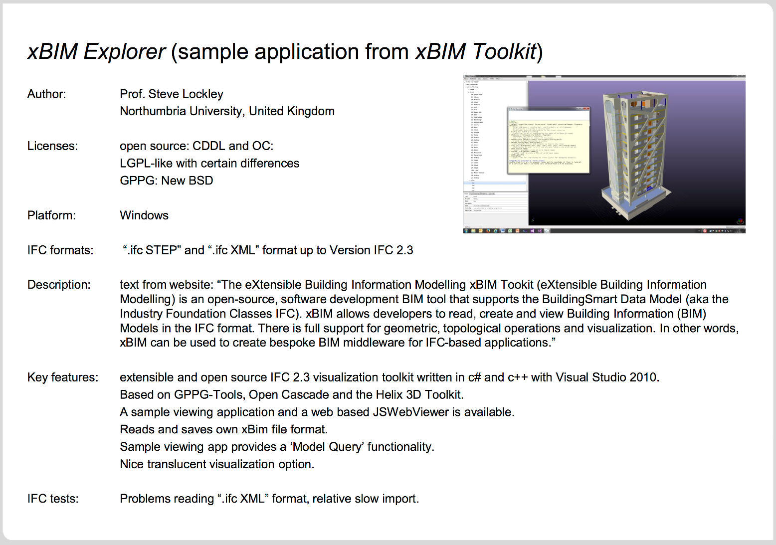
Fig. 7.3 Brief technical description of the XBIM tool
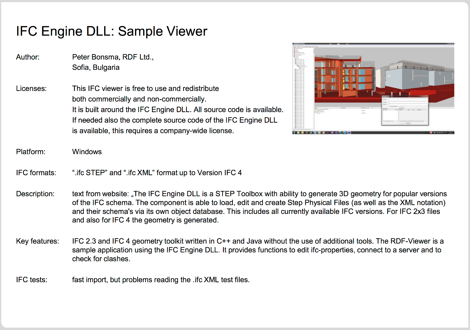
Fig. 7.4 Brief technical description of the IFC Engine DLL Toolkit
For the development of the Annex 60 model checking tool (ref Section 7.4.3) the second tool was selected due to its simpler enhancement possibilities.
7.3. Importing BIM Data to BPS
This section describes the transformation from Building Information Modeling to Building Performance Simulation in Modelica. Starting with a first and initial draft of the data transformation process adopted in this Annex, requirements for BPS in different stages of the building design are described. We detail the possibilities and requirements to generate Building Information Models with a focus on BPS in this section. The section further illustrates how to extract related information from a BIM and transforming it to be used as basis for BPS, respectively.
The use of Building Information Modeling implies interoperability between software applications and the collaboration of different disciplines. Fig. 7.5 illustrates the process how to derive Modelica models for different Modelica libraries from BIM. Each step requires different actors and software. The architect and HVAC engineer use domain specific BIM-based CAD software and may export their models to an Industrial Foundation Classes (IFC) file (left side). This file is converted into SimXML which is the file format for SimModel, a data model for the simulation domain. SimModel extends information provided by IFC with simulation specific parameters. The SimXML file is then converted to a valid Modelica model with the software framework developed in this Annex. This framework is setup to support multiple Modelica libraries as well.
This section puts energy modeling into the context of Building Information Modeling, including IFC, SimModel and tools to check the BIM for integrity.
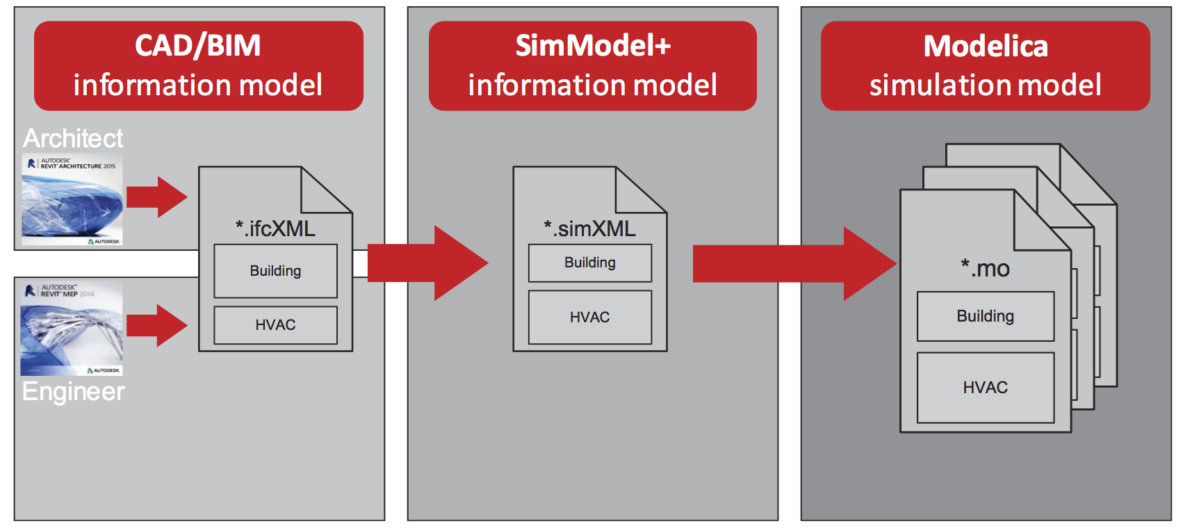
Fig. 7.5 Overview of the transformation process from IFC to Modelica models using different Modelica libraries.
7.3.1. Overall Transformation Process
For the task of converting BIM into Modelica models (as outlined in Section 7.1), we used a case study approach for the development of the tool chain (Section 7.4).
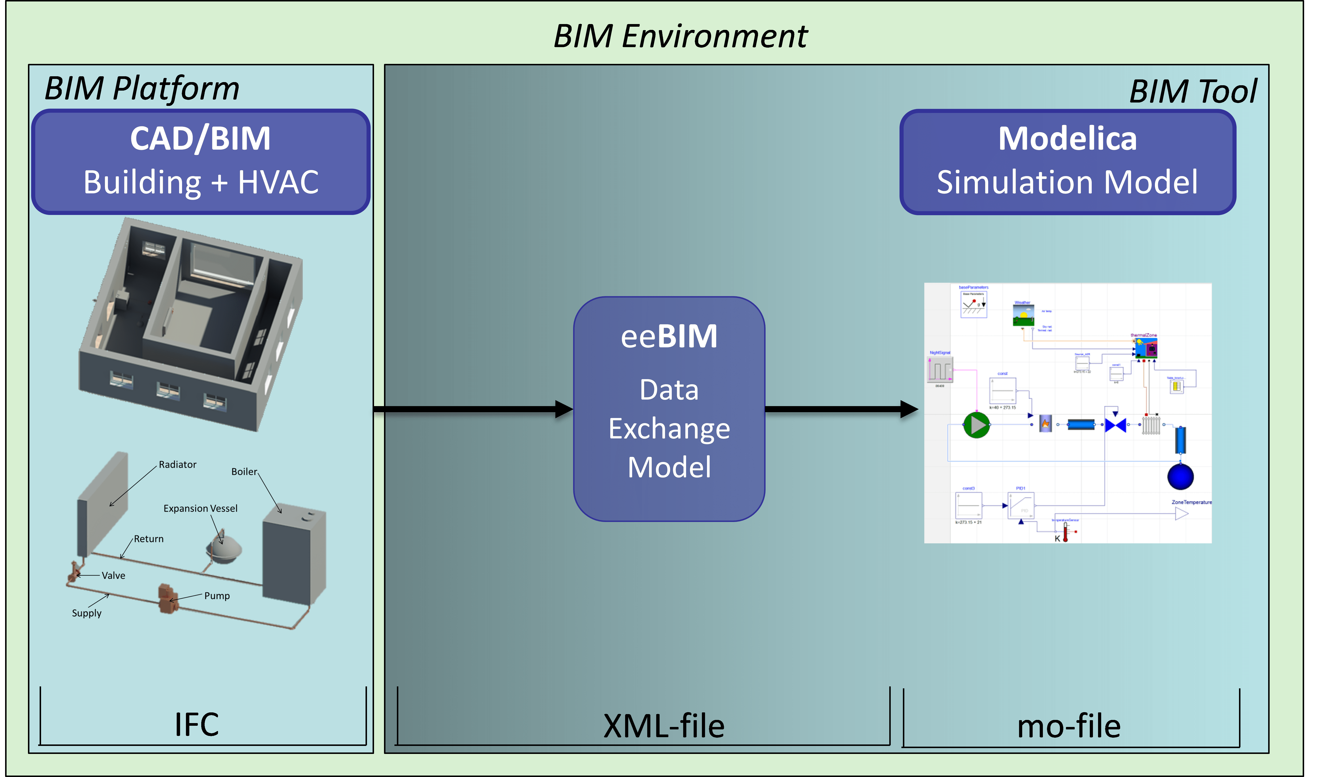
Fig. 7.6 Data transformation from BIM to Modelica
Fig. 7.6 illustrates the data transformation process within the developed methodology, in which the IFC data model is instantiated in the BIM Platform and exported as an IFC4 file. In order to read and operate with these data, the model is converted into a specific exchange model for BPS. SimModel is such a data exchange model specifically developed for BPS and thus serves as the intermediate format to support the exchange of data from BIM to Modelica in this Annex. SimModel offers a flexible data model allowing enhancements and additions as described in Section 7.3.6. The final process in the tool chain generates a Modelica file.
The conceptual and software development of this methodology was driven by a set of simple use cases (described in Section 7.5).
7.3.2. Requirements for BPS Models Across Different Stages of the Building Design Process Based on Uncertainty
BPS models can be used at different stages of the design process, for example to investigate the thermal comfort and energy consumption of a building or to support the planning of the HVAC configuration and controls. Depending on the respective application of a BPS model and the corresponding design phase, different requirements must be satisfied in terms of the nature of the model and the associated input data.
It is important to know the level of detail which is required at each design stage. This allows for the BPS engineer to generate reliable results. Here, it has to be taken into account that simulation results always comprise some extent of uncertainty. This uncertainty arises due to unknowns within the inputs of the simulation model. Certain input uncertainties decrease in the course of the design process, particularly as detailed planning proceeds and available information is increasing. Other input uncertainties are more or less constant over the entire planning process, for example: climate conditions or user behavior. The challenge is to identify which level of detail, represented by subsets of data contained in the BIM, is necessary for a BPS model at a specific stage of the design, which is a crucial consideration given the corresponding uncertainties at that stage.
To provide answers to this challenge, methods for uncertainty and sensitivity analysis can be used. In [BJH10] a methodology is described which allows for consideration and evaluation of uncertainties in BPS models using Modelica. Additionally, the methodology can be used to determine the impact of the uncertain inputs on the output uncertainty (sensitivity analysis) and, thus provides a means to rank model inputs according to their relative importance in terms of the simulation result. The most sensitive inputs are highly relevant for providing valuable simulation results while less sensitive inputs (lowest ranking) have little influence on the simulation results.
| Parameter | Unit | Minimum | Maximum | Distribution |
|---|---|---|---|---|
| zoneParam.RRest | K/W | 0.03 | 0.05 | uniform |
| zoneParam.R1o | K/W | 0.0003 | 0.005 | uniform |
| zoneParam.C1o | J/K | 1.0e06 | 2.0e06 | uniform |
| zoneParam.Aw | m² | 5 | 9 | uniform |
| zoneParam.g | 0.5 | 0.7 | uniform | |
| pipe.dp | Pa | 5000 | 20000 | uniform |
| valve.dp | Pa | 5000 | 20000 | uniform |
| flow.temperature | °C | 70 | 90 | uniform |
Accordingly, one can argue that a simulation model should account for the most sensitive inputs (even if the respective inputs are not exactly known) with respect to the output of interest. Less sensitive inputs can be initialized with default values or ignored in the model.
In the following, the procedure for uncertainty and sensitivity analysis is briefly explained and illustrated using the example of use case 1.1 (Section 7.5.1) (standard office building modeled as a simple zone with radiators and a boiler). From the results of this type of analysis one can estimate the output uncertainties and deduce BPS model requirements for different design stages.
The first step is to identify the uncertain model input parameters and estimate their respective distributions. Here, we assume that building parameters are not fully known, which leads to uncertainties in the heat demand, and the exact HVAC layout has not been specified yet. This situation can, for example, appear in the outline planning when first simulations are run, in order to support code compliance or later certifications, while significant uncertainties have to be considered.
The assumed input parameter distributions are shown in Table 7.1. Here, the first five lines correspond to building (zone) parameters, while the last three lines correspond to HVAC parameters. RRest, R1o and C1o describe thermal resistances and a thermal capacity in the reduced order building model according to VD16020. These parameters cannot be directly related to physical quantities in the building, but represent aggregates. Aw and g denote the area and the solar transmittance of the windows, respectively. The parameters valve.dp and pipe.dp are associated with the pressure losses of valves and pipes.
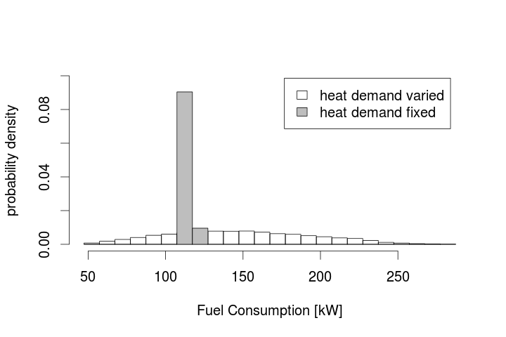
Fig. 7.7 Distribution of the fuel consumption over all simulation runs. White bars correspond to a varied heat demand according to the building parameter distributions given in Table 7.1. Gray bars correspond to a fixed heat demand and only HVAC parameters are varied according to Table 7.1.
Then, Monte Carlo Simulations are performed, where for each uncertain input parameter 4096 random samples from the given range are chosen. The simulation period is six weeks, starting from 1st of January. The considered output is the total energy consumption of the HVAC system which consists of the fuel consumption of the boiler and the electricity consumption of the pump, summed over the simulation period.
Fig. 7.7 and Fig. 7.8 show the resulting distributions of the outputs, fuel consumption and pump power, when the input parameters are varied according to Table 7.1 (white bars). For comparison, the corresponding distributions are shown when the heat demand is assumed to be known (associated with fixed building parameters) and only the HVAC parameters are varied (gray bars). It can be seen that the uncertainty in heat demand has major influence on the total energy consumption: the estimate of the total energy consumption is much more precise when the heat demand is known. The remaining, relatively small, uncertainty if the heat demand is fixed results from the uncertainties in the HVAC layout. In comparison to the building parameters, the HVAC layout plays a negligible role for the overall output uncertainty.
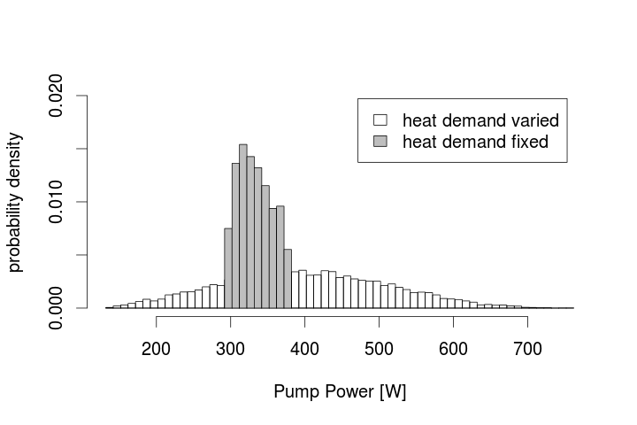
Fig. 7.8 Distribution of the pump power over all simulation runs. White bars correspond to a varied heat demand according to the building parameter distributions given in Table 7.1. Gray bars correspond to a fixed heat demand and only HVAC parameters are varied according to Table 7.1.
This effect can be quantified via the calculation of sensitivity indices. The variance-based first order sensitivity indices for all varied input parameters with respect to fuel consumption and pump power are shown in Fig. 7.9. A higher index indicates a greater influence on the observed output uncertainty. Also from this figure, it becomes clear that, in this setting, the building parameters have a greater impact on the energy consumption than the HVAC layout. In particular, the thermal resistance parameter of the simplified zone model and the window area turn out to be most influential.
So, one can deduce from these results that for a reliable estimate of the energy consumption the heat demand should be known relatively well, while a rough picture of the HVAC system configuration is sufficient at this stage. When it comes to optimizing the operation of the HVAC system, having eliminated other uncertainties to large extent, the exact HVAC layout becomes important.
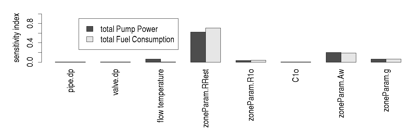
Fig. 7.9 Sensitivity indices for the outputs fuel consumption and pump power with respect to the varied input parameters. The variation of the building parameters has much more effect on the outputs than the variation of the parameters concerning the HVAC layout.
In a similar way, one can identify the following model requirements, based on the simple use case 1.1 (Section 7.5.1), for four different design stages:
7.3.2.1. Preliminary Planning
A simple building simulation model is used to estimate the energy demand of the designed building. Uncertainties in weather conditions, internal loads and building parameters (e.g. materials, areas) have to be taken into account. The resulting energy demand yields a probability distribution.
The resulting energy demand distribution from the building simulation is used to perform an HVAC simulation and to support the HVAC planning. Therefore, a simple HVAC model is used which only comprises the boiler and radiator, and yet uses the uncertain energy demand as input. If applicable, several different HVAC concepts with alternative heat sources or heat exchangers are compared. A first estimate of the energy consumption in terms of a probability distribution is provided.
7.3.2.2. Outline Planning
As more details concerning the building geometry and the materials are known, a corresponding building simulation yields a more precise heat demand, which, however, still comprises some uncertainty due to unknown internal loads and weather conditions.
An HVAC simulation is used to determine the optimal dimensions for the boiler and radiator. Uncertain heat demand, unknown set values and controls have to be taken into account. A model-based optimization of set values (e.g. flow temperatures) and controls (e.g. night set-back) could be pursued. As a result of the HVAC simulation, the estimated energy consumption is obtained and serves as a basis for code compliance and certification.
7.3.2.3. Detailed Planning
A detailed HVAC simulation is used to optimize the HVAC configuration and controls. Pipes and valves are included in the model. Uncertain heat demand, unknown pressure and heat losses are taken into account. As a result of the HVAC simulation a more precise distribution of energy consumption is obtained and serves as a baseline for building operation.
7.3.2.4. Operation Phase
A detailed as-built building and HVAC simulation model is calibrated with measurement data. The calibrated model is used for model-based on-line fault detection and optimization or model-based control.
The BPS model requirements for this simple example arise from a sensitivity analysis. For more elaborated systems with storage and renewable energy usage the picture could change slightly. In particular, controls would have a more important role to play during the early design as they tend to have a large impact on the energy consumption of innovative or low energy systems.
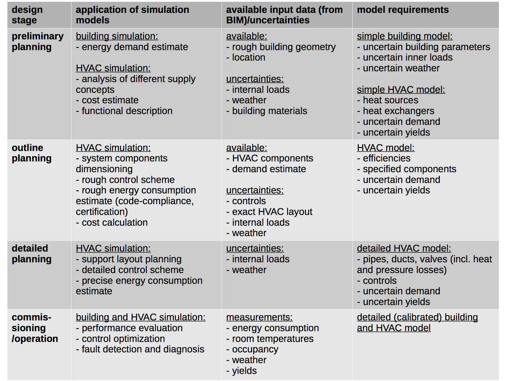
Fig. 7.10 Overview of the usage and requirements of simulation models in different design stages.
An overview of the use of simulation models in different design stages is given in Fig. 7.10, as is the availability of relevant input data for each respective phase and the data requirements for the BPS model. Although this representation is not exhaustive and can certainly not be applied to all building processes, the image indicates typical dependencies between available information and targeted BPS results. As a result, this information can serve as a basis for Information Delivery Manuals (IDM) as described in sub:numref:sec_IDM.
7.3.3. Building Geometry Generation and Processing
Building geometry definitions for use in Building Energy Performance (BEP) simulation modeling usually originate in CAD software. They are defined by CAD in 2D, 2.5D or 3D, and are delivered in electronic form or on paper.
Geometry information on paper (drawing prints) generated by 2D CAD tools, such as AutoCAD [Aut16], must be manually transcribed into electronic geometry definitions that can be read by BEP simulation programs and engines. This is a very tedious, time-consuming, frustrating and extremely error-prone process that can, depending on the size and complexity of the modeled building, consume more than a half of the total simulation project budget.
If the 2D building geometry is available in electronic format (DWG or DXF) which contains scalable dimension information, the transcription into geometry definitions readable by BEP simulation programs and engines can be a bit faster (using copy-and-past) and somewhat more efficient. Still, the transcription requires heavy human modeler involvement.
State-of-the-art 2D CAD software, such as AutoCAD, can provide the third dimension by extruding the information defined in 2D plans vertically. Such geometry is called 2.5D, as it is not true 3D geometry. While 2.5D geometry can further expedite the geometry transcription for use in BEP simulation, it can have the opposite effect when different adjacent buildings have different extrusion length.
“Model-based” architectural CAD tools, such as Revit [Aut15], ArchiCAD [Gra16], Allplan [Nem16] and MicroStation [Ben15], offer definition of building geometry in true 3D formats – geometry definitions that are object-oriented. Each of these CAD tools exports geometry in its own proprietary file format, but also includes utilities for export and import of geometry in IFC format. Third party software, such as the Space Boundary Tool [RB13] and Simergy [Alc16], can automatically or semi- automatically transcribe geometry defined in IFC format into input for EnergyPlus. Bentley’s AECOsim Building Designer [Ben15], transcribes building geometry originally created by MicroStation for seamless use in EnergyPlus. The OpenStudio platform can import building geometry defined by SketchUp (not a “model-based” CAD tool) or other CAD tools that export geometry in gbXML format [GbX16] and use it directly in EnergyPlus without any additional transcription.
Most CAD tools allow the modeler to define “center-line” building geometry models in which walls, floor slabs, ceiling slabs, roof slabs, windows and doors are represented by flat surfaces parallel to the sides and placed in the center of each particular object; “center-line” representations have no thickness. While “center-line” modeling simplifies the modeling process and may save time, “center-line” geometry definitions result in BEP simulation results that significantly overestimate building energy consumption [BMNG16].
Building geometry definitions as required for use in detailed Modelica geometry algorithms should be as precise as possible. Any current high-end “model-based” CAD tool can facilitate the necessary modeling precision; it is up to the modelers to define building geometry precisely [BMNG16]. Thus it is paramount to always verify the correctness and precision of any generated building geometry.
7.3.4. Energy Modeling Using IFC
IFC based BIM has the potential to provide significant other inputs for BPS modeling, thus reducing the time, effort and expense associated with model creation [RB13][vTR06]. To date the majority of work in the area of BIM to BPS has focused on geometry transformations [Sim15][GLG+15][Gra11][JKC+16][JS16][OMR+13]. Commercial BPS tools such as RIUSKA [Gra11][LOK10], Simergy [SHS+11], IDA-ICE [Sim15] and TRNSYS [CRR+11] focus mainly on the import of geometrical information. Section 7.3.3 describes geometry transformations in detail but such transformations require high quality IFC models which are typically not delivered in practice. Previous efforts such as the Design BIM 2010 ([BDA12]) MVD development did go beyond just geometry data, in adding internal loads data as well as high level data on space requirements and HVAC systems (CDB2010 is supported by Simergy).
In addition to geometric information, HVAC, controls, operating schedules and simulation parameters should be contained within a BIM. However, when mapping HVAC systems to BPS tools, a number of complex and interrelated issues arise. Primarily, the broad variation in representation of HVAC systems within software tools results in bespoke mapping solutions from BIM to each target BPS engine. As an example, HVAC duct designers typically use a supply and return convention for loop structure while EnergyPlus uses a supply and demand loop structure. Modelica on the other hand, only requires system topology information and a different parameter set compared to parameters typically entered by HVAC system designers.
At the data level, many of the objects required for BPS are not contained within IFC based BIM or are not inserted into IFC by appropriate BIM based CAD tools. This shortcoming is particularly noticeable in the HVAC controls domain where the object and property definitions required by simulation are not yet rigorously defined and have not been in focus of data exchange developments. As a result a formal definition of the data requirements for BPS would significantly assist data transfer to the BPS domain and MVD is an ideal platform to service this need.
7.3.5. Model View Definition (MVD) for Energy Related BIM Support
In order to facilitate data exchange between applications using the IFC schema, an MVD was developed to meet the requirements needed by BPS tools. The MVD focuses on the definition of IFC entities, attributes, relations and properties that satisfy this specific exchange scenario. This defines a subset of the building product model schema that provides a complete representation of the information concepts needed for a particular use case in an AEC/FM workflow [PWM+16].
The MVD also defines the business rules and agreements necessary to assist the implementation of import and export functions by BIM applications. Thus, a first quality assurance can be done by checking for mandatory entities and property sets. In cases where information is not currently represented in the IFC specification, properties can be defined to extend the IFC schema.
7.3.5.1. Available MVDs and Current Status
In 2016, buildingSMART published the IFC4 Addendum 2 (IFC4 Add 2), together with two new MVDs to support IFC4 implementation: Reference View (RV) and Design Transfer View (DTV). The main purpose of the first one is to define a standardized subset of the schema that supports exchange in one direction only. The RV is characterized by the ability to provide workflow for the widest array of software applications. The second MVD proposed is an extension of the Reference View. Contrary to the RV, the DTV enables model editing by design software platforms. DTV is considered the successor of the former IFC2x3 Coordination View and is compatible with IFC2x3 import [Bui16].
Since the introduction of the MVD concept, organizations started developing their own MVDs to support internal processes based on the IFC2x3 schema. There are some related to energy performance such as: Holistic Energy Efficiency Simulation and Management of Public Use Facilities HESMOS [LSW+13] and Concept Design BIM 2010 (CDB) [BDA12]. Fig. 7.11 shows a short comparison of the energy related MVDs. The HESMOS project did actually not define an MVD, the project focused on the definition of exchange requirements (ER) only. HESMOS and CDB focused on the building envelope, but added some additional HVAC related data as a first step towards a simulation MVD. CDB MVD requires 2nd level space boundaries, whereas HESMOS only demands first level space boundaries. The HESMOS project developed a conversion tool that transforms from 1st into 2nd level space boundaries. Both projects attached the internal loads to a space. HESMOS covers most of the relevant data for a static simulation, whereas CDB’s focus lays on a more general definition of the energy analysis zone. HVAC systems are only described as existing flags or with basic parameters. HVAC components itself are completely missing. In addition to that, renewables like photovoltaic components are part of the simplified definitions.
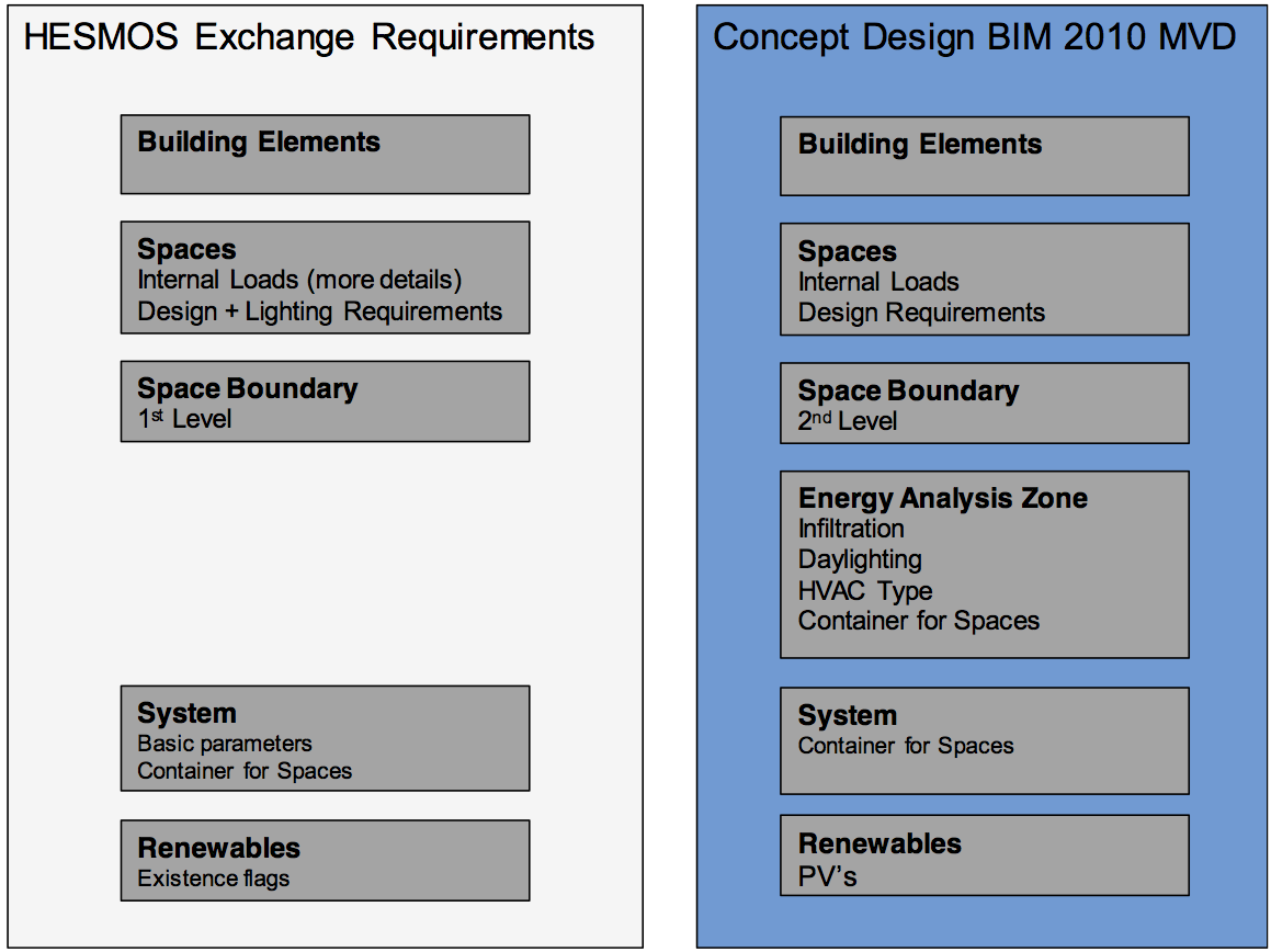
Fig. 7.11 Contrasting juxtaposition of existing energy related ER/ MVDs.
7.3.5.2. Identification of Data Requirements and Mapping to IFC
As shown in Section 7.3.2, the exchange requirements for energy simulation can be different at different stages of the building life cycle. Within this project, several use cases were defined using different levels of complexity from a single room to a large commercial building. The main purpose of creating these use cases is to analyze several HVAC systems that are used in the building sector. Based on these use cases, it is possible to identify the scope of information needed by BPS tools and subsequently map it to the IFC schema. This process involves the IDM methodology (Section 7.4.1), which is a standardized methodology to create information exchange requirements [WK10].
Working with proprietary software to generate IFC files we were bound to the content it offers. In this project, we used mainly the IFC4 version due to its added content in the HVAC component area. During the runtime of the Annex 60 project, only limited IFC functionality existed since official buildingSMART certification of IFC4 was not yet available. Through our cooperation with software vendors during the project significant effort is put into the support of IFC4 export. Over time better support for IFC4 will become available. Besides these described difficulties originating in the early stage of the implementation of the IFC4 data model, this also provides an opportunity for feedback and possible influence on further development.
In general, new versions of the IFC schema provide new entities to cover the wider scope and support additional areas of the AEC industry. Along with new entities, existing entities can change and in special cases even be deprecated. These changes have to be incorporated into the import and export functionalities of software which is then submitted for certification. Additionally, IFC supports property sets for the export of product characteristics. Some tools support these property sets with corresponding library objects, while other tools may only provide the properties through manual input. Once certified, a detailed certification report can be found on the buildingSMART website listing the level of support for individual entities.
7.3.5.3. Specification of the MVD
An MVD is composed of the following elements: ModelView, ConceptRoots, ExchangeRequirements, ConceptTemplates and Concepts. The ModelView is the description of an MVD and is specific to an IFC schema release. It groups zero-to-many ExchangeRequirements and ConceptRoots thereby defining the scope of the MVD. The ExchangeRequirements define the information necessary for a particular exchange scenario and may add additional constraints to the use of Concepts. The ConceptRoot is represented by a collection of available Concepts, each of which references a specific IFC entity, e.g. IfcSpace. Each Concept describes rules for common subsets of information (e.g. space attributes) within the context of the particular root. The Concept is backed by a ConceptTemplate describing a graph of object instances, relationships and constraints. The information contained inside of the ConceptTemplate enables the generation of instance diagrams of the MVD [CLW13]. The MVD is defined by using the open source tool ‘IFC Documentation Generator’, provided by buildingSMART ([bib]). The information defined in the existing energy related MVDs are integrated in the creating of the new MVD.
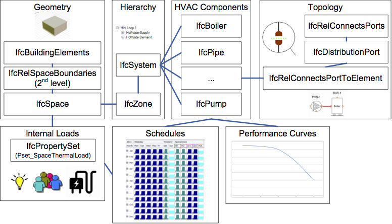
Fig. 7.12 Overview of the main topics to define the energy related MVD.
The fundamental elements for an energy related MVD are shown in Fig. 7.12.
Geometry: The Geometry defines the basis of the model. Second level space boundaries link spaces to building elements and are used as basic surfaces for the heat transfer between spaces internally and between spaces and the outdoor. These should be well defined and correct (see also Section 7.4.3.1).
Internal loads: Space contains the definition of the internal loads as property sets. IFC4 already has designated properties for internal loads as follows:
- Maximum/Minimum temperature of the space
- Maximal number of people
- The total sensible heat or energy gained
- Lighting loads
- Percent of sensible load to radiant heat
These simplified properties originate from earlier MVDs. Most importantly the dynamic nature of schedules is hereby missing which is crucial for BPS. Schedules in general are discussed next.
Schedules: The ability to define complex schedules in combination with the already defined properties allows for example the definition of detailed internal loads. BPS defines this schedule requirement that has not been introduced by other disciplines. Currently in IFC, schedules can be defined in three different ways:
- IfcWorkCalendar: On/off status through the year with predefined patterns
- IfcRegularTimeSeries: A regular time series that defines values based on a regular time interval (e.g., hourly).
- IfcIrregularTimeSeries: A time series that defines values on a irregular time series.
Typically, schedules for BPS follow a regular pattern, mostly daily, weekly and seasonal patterns are used. The ability to define patterns would simplify and reduce the data representation of schedule significantly. The IfcWorkCalender uses the IfcRecurrancePattern that is able to define such patterns, but can only contain an on/off signal and no values. For example, the presence of a certain number of people in the thermal zone on a weekday, which changes over the course of the day, or the opening range of a valve on a national holiday cannot be described with a Boolean flag. This is a significant limitation of the IFC model and creates the need for a workaround solution.
In order to enable the definition of these schedules, it is necessary to define a new concept. The IFC Documentation Generator (IfcDoc tool) is used to define the new concepts, based on the newest IFC4 data model. The top level of the concepts hierarchy is IfcObject. IfcObject is best suited for applying schedules to each possible spatial and non spatial element, such as a zone, space or HVAC component. The object is assigned via a relating control to the IfcPerformanceHistory. IfcPerformanceHistory offers the recurrence patterns, using the entity IfcWorkCalender. IfcPerformanceHistory is also defined by properties, which in turn allow the definition of complex properties and ir/regular time series. If IFC 4 allows the definition of recurrence patterns for time series, the application of detailed schedules on an hour basis over the course of a day is possible. To improve this limitation, we suggested changes for the coming version of the IFC data model. The application of this concept allows for dynamic simulation using detailed schedules of the typically complex properties for a thermal zone.
Hierarchy: The hierarchy for the thermal zones is defined using the composition concept, provided by buildingSMART. IfcSpace is the lowest level, composed to IfcBuildingStorey, which is in turn composed of IfcBuilding. IfcZone is used as a grouping mechanism, which allows for a definition of the thermal zones in combination with the space boundaries. The HVAC system is defined using IfcSystem as a top hierarchy entity. The system can be separated into subsystems. For a single loop heating system, the distribution system would be defined as supply and return pipe systems in which the radiators represent a thermal sink and the boiler a thermal source, which are also part of the subsystems. No previous agreements exist on the hierarchy of systems that is why we are proposing a simple hierarchy with one parent system for each loop that contains a supply and demand subsystem. For simulation purposes this differentiation can be useful to know which components are supplying a loop and which are demanding cooling or heating needs.
HVAC components: In the latest IFC4 version, several enhancements to the HVAC component were made. In particular, components definitions became more detailed. E.g., an IfcBoiler used to be a generic IfcEnergyConversionDevice. This great enhancement makes the representation of HVAC component more explicit. However, there are a number of HVAC component that did not get a more detailed class, such as heat pumps and combined heat and power units. Those need to be represented with a more generic class IfcUnitaryEquipment.
Topology: Since most HVAC systems are based on some kind of fluid flow, topology connections are one of the key concepts to consider. In IFC this is done by defining an IfcDistributionPort, which is connected to a IfcDistributionElement. The IfcRelConnectsPorts relationship connects two ports and forms the basis for the topology.
Performance curves: Another aspect of HVAC components are performance curves. Typically, performance curves are used to describe specific behavior of a component at varying conditions. E.g., a boiler efficiency curve that depends on the water return temperature. In IFC4 this concept does not exist. We did realize the definition of performance curves with the use of IfcComplexProperties which in turn is a list of IfcProperties. This list of properties then defines the coefficients of the curve, minimum and maximum values as well as other relevant properties.
Fig. 7.13 Overview of the concepts used to define the MVD for use case 1.1.
The developed MVD is based on well-defined ConceptTemplates provided by buildingSMART [bia]. For instance, the definition of properties and connections of HVAC components were defined using ConceptTemplates such as “Port Nesting” and “Property Sets for Objects”. Fig. 7.13 shows the concepts applied to a subset of the MVD. On the left hand side are the objects listed that are used for the use case 1.1. The top shows a list of the used concepts for the MVD. The white boxes show that the concepts can be applied to the object and the grey boxes show that the concepts are not applicable. As already mentioned the 2nd level space boundaries are mandatory for the MVD and this concept is assigned to IfcSpace. The concepts “Port Connectivity” and “Port Nesting” are necessary to connect the Ports on distribution elements and to define placement, indicating the position and outward orientation. The different materials of the numerous entities are also defined using the given concepts, such as “Material Layer Set” or “Material Constituent”. If something is undefinable using this method, an Implementer Agreement can be used (see Section 7.2.3).
It is important to notice that the process of certification is done on the basis of MVDs and not the general IFC schema. This process requires time and depends on buildingSMART as well as software developers. However, there is already some work being done to provide IFC4 support within 2016.
7.3.5.4. Outlook
The MVD developed in the Annex 60 project applies the methodology from buildingSMART, and uses the recommended ifcDoc tool for its formal and descriptive definition. IfcDoc enables the export of HTML documentation in the mvdXML format (official BSI format) for software certification and the generation of a subset schema containing all relevant entities and properties of our MVD.
Available ConceptTemplates are re-used as far as possible. While it covers all requirements identified by the various use cases, the MVD has been designed to be a general purpose view for thermal simulations, i.e. it is not restricted to the Modelica simulation package. Since the MVD is developed based on our set of use cases it has a limited scope in terms of HVAC objects, but it contains all key concepts related to BPS. Feedback on what is missing in the IFC4 data model from a BPS perspective as well as a description and discussion of key concepts and issues form important steps towards a first BPS MVD.
Besides the MVD itself, we also discovered a number of inconsistencies or missing concepts in the IFC data model.
- Missing pattern definition for schedules
- Missing explicit classes for heat pumps and CHPs
- Missing performance curve concept
- Missing agreement on system hierarchy
The next step will be to submit the MVD proposal to buildingSMART for further review by the community as well as to extend its scope to cover all relevant HVAC objects. As the current proposal already includes definitions from previous work, in particular the space boundary add-on view to fill the current generic simulation MVD gap. In parallel to the review period the software certification process can be prepared, which means to specify test cases and expected quality criteria. For this, the developed use cases and prepared example data can be used as a starting point. They already cover the main aspects of our use cases, but may need to be extended to check further aspects of the MVD.
7.3.6. SimModel: A Data Model for BPS
SimModel is primarily used as an internal data model by the Simergy software developed at LBNL and continued by Digital Alchemy [LBN13][SHS+11]. This tool was first conceived as a platform that facilitates data flow to and from BPS simulation tools to and from potentially any building modeling tool [BMR+11]. Bi-directional data flow is possible to and from IFC BIM, DOE-2 software or tools that use the DOE-2 engine, EnergyPlus, and tools with gbXML export (Fig. 7.14). These tools are typically used for BPS simulations. Data from any of these environments can be mapped to and from the SimModel data model using the Simergy software [LBN13].
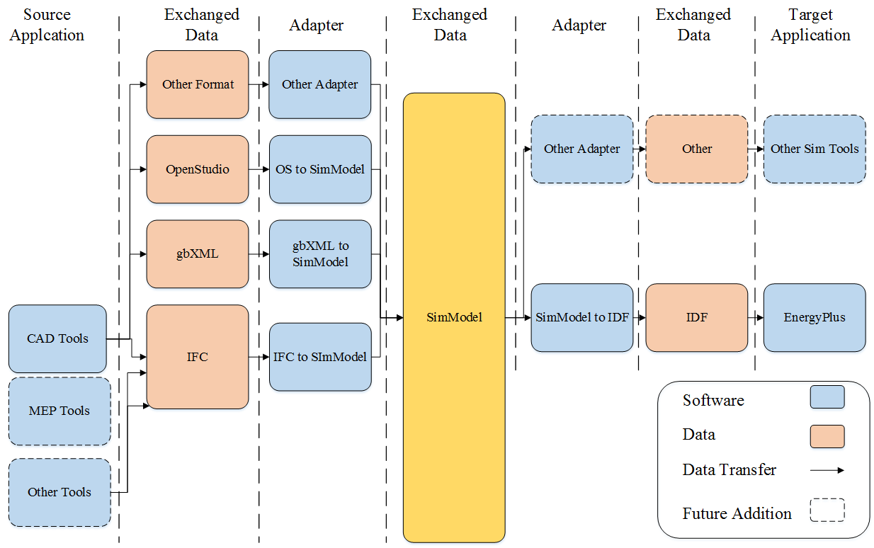
Fig. 7.14 Interoperable data exchange enabled by SimModel. This solution enables re-use of original project data as contained in IFC based BIM (bi-directional mapping) and data from other sources (import only)
SimModel is an object-oriented data model which defines all object /attribute/relationship sets used for BPS. The primary objective of SimModel is to accommodate the existing input data requirement of EnergyPlus, while allowing mapping from/to other domain data models and easy incorporation of new definitions [BMOD+11]. At its core, SimModel is represented using the XML markup language [OSM+11]. This representation is closely aligned to the IFC data model, in order to link to incoming or outgoing IFC information (Fig. 7.14), a motivating factor for using SimModel in this project. In this context, SimModel also reduces some of the complexity of the IFC data model by simplifying relationship objects though direct object references.
7.3.6.1. SimModel Design
SimModel incorporates a number of features that address current domain weaknesses (as detailed in [OSM+11]), a set of requirements for a shared simulations model and is easily extensible to account for future domain advances. This data model ensures interoperable exchange of simulation data within the simulation domain and most importantly across an entire building project. The unique design enables interoperable data exchange and uses a number of features to do so, these include: mappings to/from existing domain models; structured yet flexible class definitions; property set definitions; object type definitions; model ontology; templates and resources. The following subsections detail only the key features.
7.3.6.2. Data Model Mappings
The data model should facilitate seamless data exchange for the extended building-simulation domain and even for the entire AECOO industry [NRE10]. Version 1.0 supports BIM concepts from IFC, gbXML, IDF, and OpenStudio [NRE10]. Version 2.0 adds support for SDD (Standards Data Dictionary) to enable the foundation for code compliance analysis (here California Title 24) ([MHS15]). The quality of data varies with each file format so customized adapters enable single or bi-directional mappings on a case-by-case basis. SimModel can also accommodate bi-directional mapping to other data models as the need arises, e.g. IDA-ICE or IES-VE.
7.3.6.3. Class Definitions
Data element/entity ontologies vary greatly between SimModel, the EnergyPlus schema called Input Data Dictionary (IDD) and gbXML. The EnergyPlus IDD contains ~650 element types and other relevant data model schemas contain several hundred classes. SimModel uses approximately 120 data model classes to represent the merger of the EnergyPlus IDD and other model schemas. This approach results in fewer software classes, less code to maintain and simplified model evolution.
The streamlined approach uses a type/subtype hierarchy for each data model class. An example best illustrates this concept. SimMaterial is a data model class that represents material types. However opaque and transparent are types within that class, where each type then contains the relevant subtypes, e.g. class = SimMaterial, type = OpaqueMaterial, subtype = NoMass.
The type/subtype approach also acts as a filter for data on an object instance to ensure that only properties relevant to the subtype are used. This approach enables schema evolution and application specific schema variants. This property filtering is a key feature that is not supported by most other data models.
7.3.6.4. Model Ontology
The SimModel ontology introduces two concepts that were previously undefined in simulation data models: 1) projects and 2) design alternatives. These new concepts enable an efficient re-use of existing data and minimize the overhead associated with tracking changes between design alternatives. Other features include geometric entities, HVAC systems, HVAC components, groups, controls, simulation parameters, and outputs. The concept of modeling systems and zones as groups is unique when compared with other data models in the simulation domain. This feature aligns with the definition of Thermal Blocks as contained in COMNET (a set of rules and procedures for energy modeling) [RES10]. Explicitly defined properties enable collections of group members. SimModel also surpasses IFC with respect to loosely defined building element assemblies by formalizing definitions for curtain walls, ramps, roofs, stairs, transportation systems, site assemblies, day-lighting assemblies and ventilation assemblies.
7.3.6.5. Resources
SimModel takes advantage of a number of resource objects that are absent from other simulation domain data models. These include actors in a project, which can include people, organizations, or people in organizations (as in IFC). Examples that have come into SimModel from CDB-2010 ([BDA12]) include the building owner, the architect, and building occupants. Actors are also used to support the fact that simulation tools require not only heat generated by occupants but also their behavior and presence. For the purposes of collaboration, applications may also associate an actor with the ownership of each individual object instance (called the OwnerHistory as in IFC). Other new resources include templates and library object entries that support the reuse of library and template content. With this model in place we now describe a transformation process from SimModel to Modelica.
7.3.6.6. Extensions
Due to the nature of SimModel, the majority of concepts, objects and parameters did already exist and could be used in this project. The project initiated the addition of a small number of parameters as well as a couple of new object subtypes. In particular, controller representations are simple in SimModel (originating in the simple representation in EnergyPlus) and needed some of these extensions. In addition, we added a couple of parameters such as area and normal direction to the space boundary object. This addition eliminated the need for 3D geometric processing for our conversion from SimModel to Modelica.
7.3.7. Formal Transformation Process
This subchapter formally describes the data transformation process mathematically.
7.3.7.1. Overall Definitions
In order to map SimModel objects and properties to relevant Modelica objects and properties, in the Annex 60 project a set of generic mapping rules was developed. This mapping of objects and parameters consists of four mapping rules using a formal mathematical description (Fig. 7.15). To illustrate the mapping appropriately, the rules are defined by using set theory [PD00]:
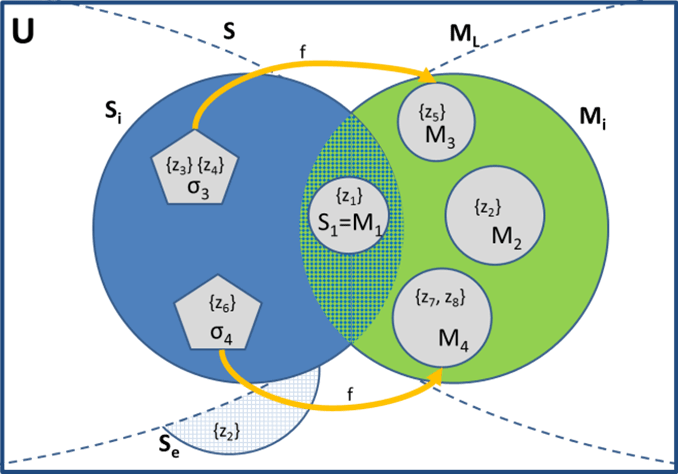
Fig. 7.15 Venn diagram for the mapping details between SimModel and Modelica
Let \(U\) be a universal set. \(U\) contains the input data for SimModel (represented by the subset \(S\)) and Modelica (represented by the subset \(M\)), where \(S\) is a subset of \(U\). It represents the SimModel objects with corresponding parameters (1).
\(S_\text{e}\) represents the extension of parameters and objects beyond the data set of SimModel (S). This is necessary for representing the required additional data within the targeted Modelica libraries (2),
\(S_\text{i} (i= 1 \dots n)\) is a subset of elements of S, where \(S_\text{i}\) contains objects and parameters as relevant input data for the targeted \(M_\text{i}\) (3) + (4),
\(z\) is an element of the set \(U\) and represents a single parameter.
\(M_\text{L} (L= AixLib, Buildings, BuildingSystem, IDEAS)\) is a subset of \(U\). \(M_\text{L}\) represents the objects and parameters necessary for a specific library in Modelica (5),
\(M_\text{i} (i= 1 \dots n)\) is a subset of \(M_\text{L}\). It represents a set of objects and parameters (7) + (8),
For an optimal communication between the two data models, the interface represents a minimum data flow. To meet this requirement, the following boundary condition needs to be fulfilled (9).
The following two sections define the formal transformation rules. Thereby, two different kinds of mappings are distinguished. The first section considers the so-called object mappings while the second section focuses on parameter mappings.
7.3.7.2. Object Mapping
The object mapping defines how a mapping between objects of the two domains essentially takes place. The type of mapping thereby depends on the issue if objects can be mapped directly (i.e., one to one), if a single object needs to be mapped to more than a single object or vice versa (referred to as many to one or one to many mapping), or if such a mapping is not possible at all (gap) which requires to extend the model, respectively.
7.3.7.2.1. One to One Mapping
The One to One mapping formally represents an intersection of \(M_\text{L}\) and \(S\) (10) and identical subsets (11):
Example: Identical fans in SimModel and Modelica.
7.3.7.2.2. Many to One (12) / One to Many Mapping (13)
Several different subsets \(S_\text{i}\) represent the necessary elements for a single \(M_\text{i}\) or vice versa
Example: A valve is part of the radiator object in SimModel whereas in the used Modelica library models the valve and radiator are separate objects.
7.3.7.2.3. Gap
The SimModel project instance does not contain the targeted object (14) and needs an extension by \(S_\text{e}\) (15) or this missing object needs to be added to the corresponding instance of the data model.
Example: A SimModel project instance does not contain an expansion vessel for hot water systems.
7.3.7.2.4. Combination
Possible combination of the above rules.
7.3.7.3. Parameter Mapping
Similar to the object mapping, model parameter need to be mapped between the two models. We formally distinguish between the following situations.
7.3.7.3.1. One to One mapping
Intersection of a subset \(S_\text{i}\) and \(M_\text{i}\) (16) with identical parameters (17)
Example: Power of a radiator (W).
7.3.7.3.2. Gap
The specific data model defined in SimModel does not contain the parameter (14), so that it needs to be extended by \(S_\text{e}\) (15) or added to this specific data model instance.
Example: A SimModel project instance does not contain the maximum pressure for a tempering valve.
7.3.7.3.3. Transformation Rule
The transformation rule represents a special case. Technically, it describes a gap, as there is no corresponding parameter in SimModel (14). However, with a transformation of a subset it is possible to create the required data. With this rule, a new subset \(\sigma\) is accordingly defined.
\(\sigma\) represents a set of parameters which are similar to the definition of parameters in \(M_\text{i}\) (18)
To accomplish the mapping with a union of \(M_\text{i}\) with \(\sigma\), it is necessary to transform the elements in \(\sigma\) via an algorithm (19)
To combine several parameters, it is necessary to define transformation algorithms (20) + (21)
The transformation rule covers a conversion of parameters as well.
For example, a simple unit conversion or a more complex conversion of one function to another function needs to be handled by a certain algorithm.
7.3.7.3.4. Combination
Possible combination of the rules above.
Fig. 7.15 exemplarly conceptualizes the mapping rules for the object mapping with the universal set \(U\), the corresponding subsets \(S\), \(M_\text{L}\) and \(S_\text{e}\), and the sub-subsets. The figure specifically illustrates the parameter mapping. \(S_\text{1}\) and \(M_\text{1}\) contain identical parameters and represent the first rule. \(M_\text{2}\) represents the gap, which is closed by embedding the missing information in the SimModel data model via \(S_\text{e}\). \(\sigma_\text{3}\) and \(M_\text{3}\) represent a transformation from many parameters in the SimModel set to a single parameter on the Modelica side. At this point, it is necessary to use the transformation rule, as the user needs to implement algorithms (illustrated by the function f) to combine the parameters. The outcome of this algorithm is a single parameter on the Modelica side. The link between \(\sigma_\text{4}\) and \(M_\text{4}\) demonstrates the use of a single parameter at the SimModel side to define multiple parameters on the Modelica side.
7.4. Open Framework for Modelica Code Generation from BIM
This subchapter presents and describes tools developed in this Annex 60 project required for the conversion from Building Information Models to Building Performance Simulation using different Modelica libraries. The tools result in a tool-chain which is highly modular and supports the reuse of different parts in follow on projects. We identify three necessary steps:
- Data model generation
- Information selection, enrichment and verification
- Simulation model generation
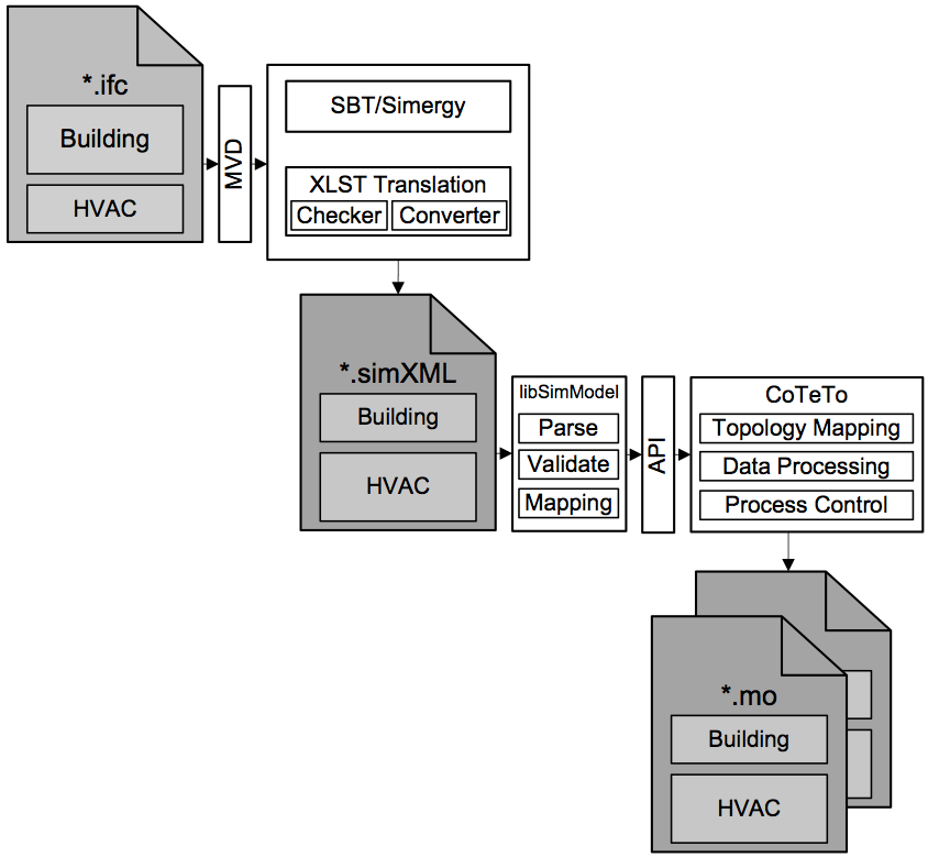
Fig. 7.16 Overview of the transformation tool-chain from IFC to SimXML and Modelica model
7.4.1. Conversion from BIM to BPS
This section details the process from BIM to Modelica models. Fig. 7.17 shows this overall process. There are three actors involved. The architect generates a geometry model, verifies its correctness and generates 2nd level space boundaries. The HVAC engineer uses this geometry model as a starting point and adds the HVAC model of the building. He also performs a validation check. The simulation team then gathers necessary data to enrich the simulation model, runs the simulation and analyzes the results. This process view illustrates the IDM (Information Delivery Manual) that goes along with the MVD defined by this project.
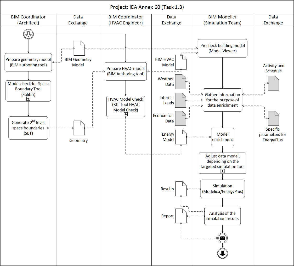
Fig. 7.17 Overall process diagram (IDM)
7.4.1.1. Data Model Generation
An obligatory requirement for the framework is a valid and well-formed BIM model. A well formed BIM in the context of BPS means the definition of geometry (e.g. different constructions and corresponding space boundaries) as well as the HVAC system. We distinguish between geometry, building physics and HVAC components as semantic model parts within a BIM. The building geometry is created with BIM-based CAD software (Fig. 7.16). Within this software physical and semantic properties of the building objects are defined as well. Based on the geometry of the building, HVAC engineers further add information about the energy system to the BIM. Using a single file format for data exchange between different actors creates added value for actors and users. However, there is need for an actor who coordinates data exchange and data migration to the model. This BIM manager requires knowledge in different domains (e.g. geometry, building physics and HVAC components) as well as in the field of data exchange. As some planning is done in parallel, the BIM manager is as well responsible for merging partial models. This is important for the overall consistency of the BIM within these collaborative activities. Model quality is highly important for the use of the presented tool-chain. We assume to start with a well formed and valid IFC file. Starting from this IFC file, the transformation process is initiated using the tools from the tool chain as shown in Fig. 7.16.
7.4.1.2. Information Selection, Enrichment and Verification
The IFC format is able to store detailed information about various disciplines, for example, fire protection. Not all of the exchanged data is needed for BPS, therefore the energy consultant uses a specific Model View Definition, which is described in Section 7.3.5, to read the relevant data for BPS in Modelica (middle part in Fig. 7.16). An MVD is a subset of the IFC-schema that defines discipline-specific exchange requirements. As an example the energy consultant needs spatial surface geometry defined in the MVD as a basis for thermal zones. On the other hand, the simulation of HVAC equipment might need further information that is not part of the information model of IFC. To store and exchange this additional information, the energy consultant migrates the collected data from the MVD to the intermediate file format SimXML. The transformation is done by using Space Boundary Tool and Simergy for the geometry part of the IFC mode, see Section 7.4.3.1 and Section 7.4.3.2. The HVAC related objects are transformed with a tool developed as part of this project. It uses the XSLT language to translate the model into SimXML (Section 7.4.3.4). The information model behind SimXML is called SimModel (see Section 7.3.6) which is a simulation domain specific data model. Both tools add further, missing information to the SimXML file. This particularly refers to space boundary and semantic information, needed for dynamic building simulation. The resulting file is automatically verified against the XML schema definition. Section 7.4.3 describes technical details of the transformation from IFC to SimModel.
7.4.1.3. Simulation Model Generation
The last step is the generation of valid Modelica code. This task divides into the parsing and validating of the SimXML file, mapping from SimModel to a specific Modelica library (e.g. BuildingSystems or AixLib) and textual output of the code itself. For parsing and validating the SimXML file we developed a C++ framework, called libSimModel (Section 7.4.4). In addition the code maps objects and parameters defined by mapping rules from SimModel to Modelica library. Furthermore, individual processing and the mapping of object topologies (as these differ in different libraries) need to be considered. Through an API we expose relevant data available in libSimModel to the Python programming language and perform these individual steps in a tool called Code Templating Tool (CoTeTo). Both object and parameter as well as the topology mapping needs to be defined by a simulation expert, who has fundamental knowledge of the considered library and SimModel. CoTeTo collects now all information and prints out Modelica code with regard to a correct Modelica syntax. The process is described in detail in Section 7.4.6.3.
7.4.2. Data Transformation
The primary role of a Building Information Model (BIM) is to serve as a comprehensive repository of data that are retrievable by multiple software applications which participate in the same AECO industry project. Data placed in a BIM by one software application are retrieved and used by other applications. Retrieved data are at times not useable by the recipient application in exactly the same form and/or format as received; in such cases the received data are manipulated and/or transformed before they can be used [BK07].
A software application is entering new data in a BIM, it is authoring those data. Such data constitute the original BIM data that can then be used by other, usually downstream, software applications. Downstream applications may, and often do, support different disciplines and have implemented different model views than the authoring application.
CAD applications generate building geometry and, in the process of documenting it, are usually the first to create original data. Additional data are subsequently authored by downstream applications. Because the need to exchange data among CAD applications is relatively infrequent, the real payoff from software interoperability is seamless data exchange with and among downstream applications. But that data exchange is not always automatic or straight forward.
A software application imports or generates itself all data it manipulates. To obtain valid results, data imported by an application must not only be in a form and format that is readable by the application, but also must represent values within the range the application expects to import. For example, if a downstream application expects to import a value for floor-to-floor space height, the imported value must represent floor-to-floor and not floor-to-ceiling space height. Because of the diversity of applications (and their internal data structures) that may participate in a given data exchange, “original” data must often be transformed before they can be used by a downstream application – data sets must be reduced and/or simplified, or data must be translated and/or interpreted.
In general, data transformation can be classified in four types:
- Data set simplification. An original data set can be too “rich” to import by a downstream application. For example, the original definition of a floor structure may include the precise geometry of all material layers in the floor, while a downstream application can only import a generalized “sandwich” definition of the floor. The redefinition of the floor “sandwich” that loses some geometry detail but still accounts for all material layers amounts to a simplification of the original geometry. Geometry approximation usually falls in this category.
- Data set reduction. If the “rich” original geometry data set contains definitions that cannot be used by the downstream application, these are omitted from the exchange set. This is the case when, for example, a column in its original is partially embedded in a wall, but the downstream application cannot import column definitions; the column definition is excluded from the exchange set and the wall of the original definition is extended over the space previously occupied by the column.
- Data set translation. Most of this type of data transformation involves units of measurement, such as conversion of metric to imperial units. Another type of translation is the textual definition of surface orientation which in the original definition is expressed by the “normal” vector, and the downstream application requires textual identification of the orientation (e.g. “exterior”).
- Data set interpretation. When data required by downstream applications have not been explicitly defined before, it may be possible to derive them from original data which themselves may not be needed by these applications. The interpretation of original information that yields derived data then becomes a process that can involve recognition, extraction, sorting, and calculation. This process can be relatively simple, as in deriving the floor-to-wall area ratio not included in the original BIM data, or fairly complicated, as in deriving the proper “net” building area as specified by local code.
Legitimate data transformation is performed following rules which are agreed upon and standardized. These rules cannot be arbitrary and should be embedded in data transformation software to be executed faithfully. Manual data transformation is acceptable only if it follows applicable rules.
7.4.3. IFC to SimModel
The process of converting the IFC data model into SimModel consists of various tools that convert both the geometry as well as the HVAC data. For the geometry, the Space Boundary Tool generates 2nd level space boundaries. Simergy will transform the geometry data from IFC to SimXML. For the HVAC data, we first describe the checking tool and then the converter.
7.4.3.1. Space Boundary Tool (SBT)
SBT is a tool that calculates all levels of space boundaries that define surface geometry which constitutes the building geometry model in BEP simulation using EnergyPlus and other simulation engines with similar internal geometry models [Baz10]. The main SBT algorithm is based on graph theory to convert a three-dimensional architectural building model without defined thermal space boundaries into geometry suitable for import into a whole-building energy performance simulation engine such as EnergyPlus [RB13]. The algorithm expects input specified as an Industry Foundation Classes (IFC) model, accepts a wide variety of input geometry, and is capable of accounting for a building’s construction material configuration as well as its geometry. The described approach is limited to solid-to-solid heat exchange; solid-to-fluid and fluid-to-fluid heat exchange is not considered.
In addition, SBT performs two other functions: It (a) automatically performs data transformation that is necessary so that EnergyPlus- like simulation engines can read and use information contained in SBT export files without further data transformation, and (b) it automatically corrects modeling errors that can be automatically corrected. All data transformation is performed according to rules embedded in SBT. The following is the list of 16 geometry data transformation rules embedded in SBT:
- Skipping of internal wall objects when walls are entirely contained within the same thermal zone;
- Reversal of the order of construction material layers for ”other side” second-level space boundaries for walls and slabs which have asymmetric construction;
- Redefinition of embedded columns as separate wall objects;
- Definition of the remaining wall construction parts when columns are only partially embedded in walls;
- Recognition of exterior building shade types;
- Positioning of exterior building shades right outside the exterior space boundaries of exterior walls;
- Detection and redefinition of virtual walls and slabs;
- Assignment of “virtual constructions” to virtual walls and slabs;
- Identification of floor and ceiling surfaces of a slab;
- Subdivision of slabs with voids into “void-free” segments;
- Redefinition of “exterior ceilings” as roofs;
- Connection of slab-on-grade objects to the ground object;
- Creation of the parent wall’s space boundaries for windows (if missing);
- Adjustment of window area to effective glass area;
- Linking of glazing definitions to Window 6.2 tool;
- Linking of material and construction objects to the EnergyPlus library of materials’ thermal properties.
SBT’s automatic model correction is limited to surface connecting errors typically prevalent in BIM geometry models generated by industry modelers: surfaces not connecting when connection is intended and/or necessary, and surfaces penetrating each other when such penetration is not intended. In modeling cases where not connecting surfaces is intentional (but SBT detects a gap between surfaces as defined in the IFC input file), SBT allows its user to set tolerance that identifies the intended gap and does not treat such instances as errors.
In addition to flat planar geometry, SBT can generate geometry models of curved surfaces and spaces. It calculates the geometry of single flat segment connections between end points of curved surfaces, but overrides surface area and space volume data associated with flat surfaces with actual values of curved surfaces and spaces. Since IFC definitions of curved surfaces is limited to 2D curves, SBT can itself only accept 2D curves. The tool can also interactively map thermal properties of construction materials from ASHRAE specifications to construction materials identified in the imported IFC geometry.
The tool generates two export files: an updated IFC file (with added space boundary definitions) and an IDF file that delineates the building’s geometry for direct input and execution in EnergyPlus. The latter exports a 3D wire-frame view of the building geometry imported into EnergyPlus, which facilitates visual inspection of correctness of the imported geometry. Section 7.5.9 shows an example of this transformation.
7.4.3.2. Simergy
Simergy is a simulation front end that currently supports EnergyPlus simulations and analysis for the California Energy Code (Title24). With its data model SimModel (Section 7.3.6) aligns closely to the IFC data model and this supports import and export of IFC files as well as other data formats (e.g., gbXML or EnergyPlus input data format (IDF)). The promise of Simergy is to allow easy reuse of data in form of library object entries as well as data and system templates. This enables quick setup of detailed simulation models that can easily be adjusted and optimized.
In context of this project and its tool chain, Simergy provides mainly two functions. The first one is the import of IFC data files and the export of SimXML files containing geometry data. For this function it can either use space boundaries generated by SBT or generate them internally. The second feature is the addition of internal loads data. While previous efforts (such as Concept Design BIM 2010, [BDA12]) tried to enable the definition of internal loads in CAD applications, currently support is only partial. Especially scheduling data is not supported by CAD applications. Since schedules are a major part of internal loads definition, we add them for this project within Simergy. Besides the geometry and internal load data, HVAC data is an important part of the simulation model and the relevant data transformation and checking is illustrated in the next subsections.
7.4.3.3. IFC Model Checking
Quality assurance of the initial BIM model has been identified as an important precondition for a qualified simulation process. Thus, the objective was to provide a coherency check of the IFC data to ensure that data entering the overall tool-chain passes quality requirements. The conception of the tool builds on existing generic software components and packages that were used to implement the tool.
7.4.3.3.1. Requirements
Section 7.3.5 highlights general requirements for quality assurance within the BIM-based processes. In the context of the BIM to Modelica conversion process the required data quality was examined in a scenario-based requirements analysis. Based on these results specific rules were derived which specify model quality and IFC contents. For example, all pipe parts of a pipe circuit have to be correctly connected (referenced). The rules aim to detect inconsistencies within the designated source data of the simulation, before they are transformed to the intermediate format SimModel.
7.4.3.3.2. Concept
The tools core architecture is based on concepts and generic components of the BLM collaboration toolKIT. There are two main underlying concepts, such as the workflow based conception of the user interface, and the concept of independant rules written in XML files to define the domain-specific model checking aspects. In order to support non-experts the UI was designed as a four-step procedure to check a model file against given rules. These rules are formalized in [EvB13] and are stored in different XML files. The rule-based method builds a base to depict the simulation-related data quality demands and enables to check whether a designated model complies with them. Primarily the defined rules in natural language have to be formalized in order to build the logical (domain-specific) base for the machine-interpretable business logic (rule code). Methodically the first step of formalizing the rules takes necessary elements of the specified IFC4 syntax on a binary level into account (e.g. paths to respective object classes). These first rule parts or elements build the base for deriving collections, resolving relations etc. as needed to formalize the overall natural language content (rule logic) into rule code. The other developed components which adopt the reused concepts, together with the new developed viewing component are finally integrated into a standalone tool. This application together with the separated rule base is available at https://download.building-lifecycle-management.de for free. The application is used to support the designated users of the projects tool-chain with respective quality measures to examine their potential IFC-based input data.
7.4.3.3.3. Implementation
The model checking tool is released using the component-based-development approach based on the .NET framework. The developed rules are either required or optional and following rules were developed for the context of the project.
Obligatory rules:
- building context information, e.g. proper hierarchy, location information
- building elements have material (layers) connected
- space entities have space boundaries connected
- all (HVAC) IFC components have to be connected to a IfcSystem (or derivate)
- air systems are connected to a thermal zone
- mechanical air systems contain at least one fan component
Optional rules:
- mechanical air systems are either fresh air or are closed loop systems
- controlled water systems contain at least one pump component
Fig. 7.18 shows the current development stage of the user interface of the standalone software tool “KIT EnEff-BIM Model Check”. The workflow of model checking is presented in four steps:
- load model file
- select rules
- execute model check
- summarize results
The workflow is displayed in a corresponding four tab view to the user. Besides the possibility to export a respective (error-) report to a spreadsheet file in tab 4, as well a call to the conversion tool has been implemented. In case of a fault free model check the already loaded and checked ifcXML model file is passed as an argument to the standalone console application Section 7.4.3.4. This converter is described in the next subsection.
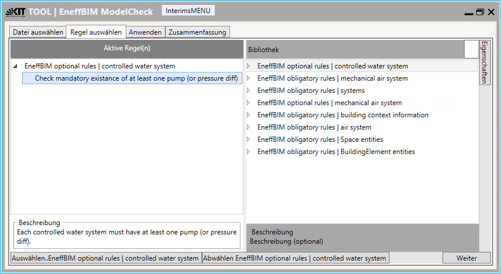
Fig. 7.18 Screenshot “KIT EnEff-BIM Model Check” Version 0.9 rule selection tab.
7.4.3.4. XSLT-Based IFC to SimXML Converter for HVAC Elements
The main objective of this tool is to provide a mechanism that converts the HVAC partial model in IFC4 to the SimModel format.
7.4.3.4.1. Requirements
For the development of the converter tool, the Annex 60 use cases define the requirements and build accordingly the logical base for the transformation of the IFC4 HVAC partial model to SimModel. The web-based BIM*Q platform ([316]) was used to collect and specify the requirements needed for the translation. The IFC entities related to the use cases and their parameters form the mapping information of the respective SimModel objects.
7.4.3.4.2. Concept
The concept of the conversion tool is based on the existing (technical) World Wide Web Consortium (W3C) approach that specifies the eXtensible Stylesheet Language (XSL) Transformations - XSLT - as a transformation technology for XML syntax. The static translation of XML-based IFC data into elements of the XML-based target format SimModel is addressed by an established, scalable and extensible solution. The core principle of the XSLT 1.0 technology can be described in four steps (cf. Fig. 7.19):
- load the source model as stream object,
- load the XSLT files (transformation templates),
- apply the templates to the source data stream and populate the emerging Result Structure Tree (RST), and
- write the RST into a designated target file.
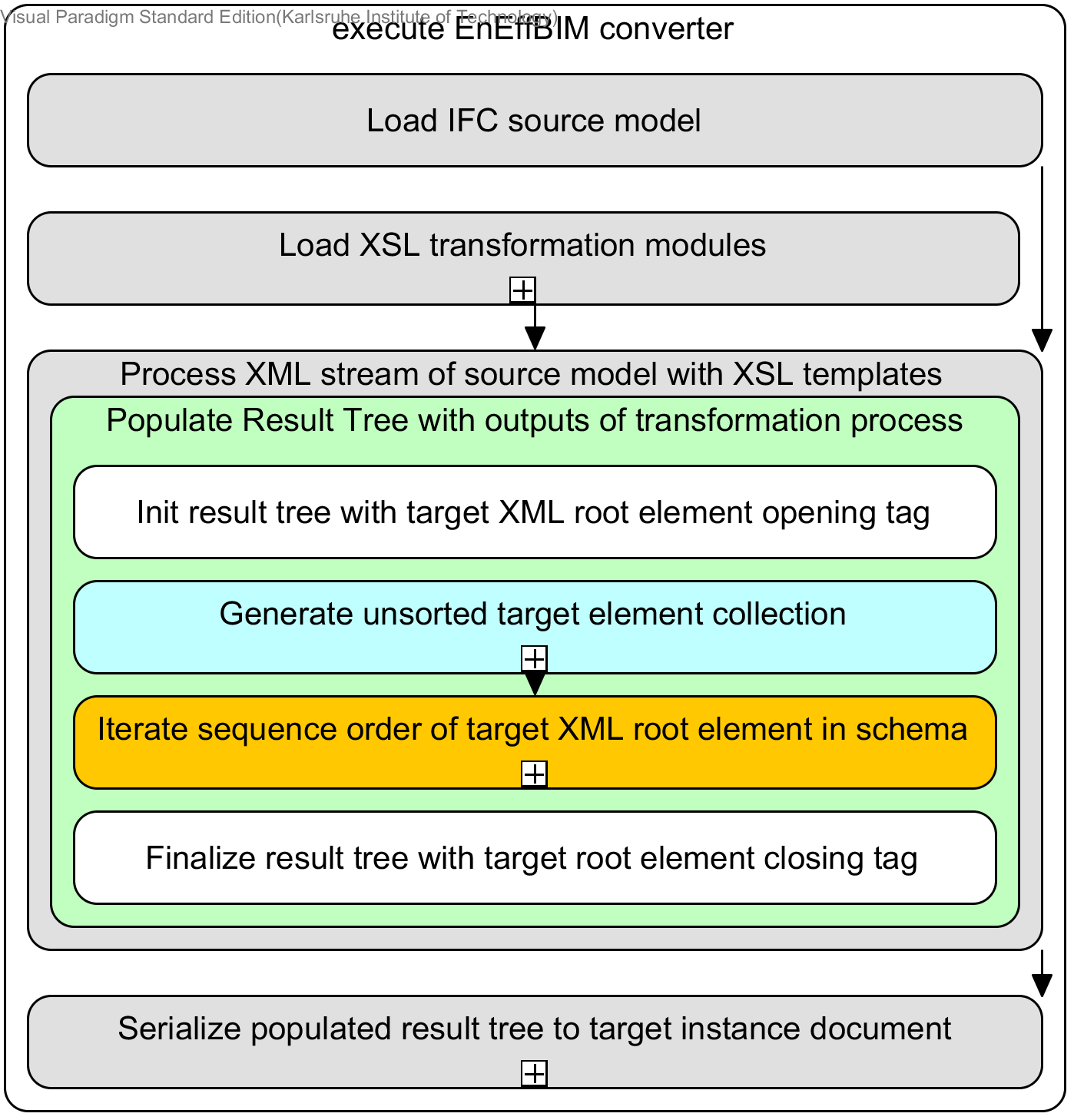
Fig. 7.19 Overview of the concept building blocks.
The static mechanism of XSLT requires an a priori definition of the exact translation instructions, and therefore persists of static templates within the framework of the XSLT application. Due to the joint development of the mapping requirements, the static approach of XSLT was supplemented with generic solutions. These are specified in the following four concept blocks that define the core architecture of the tool:
- Prefilter the relevant IFC model entities from the source model data stream. Several “Traversing Templates” (for processing the IFC topology) are used on side of the technical development to optimize the overall conversion procedure (in the subsection “Implementation” we describe how this concept block is realised and how to bypass it)
- Dynamic injection of the externally defined translation instructions between source and target model (the used concept of a simple syntax for the mapping logic is introduced in the following sub-section)
- Trigger the (element-wise) generation of the target model contents by starting the conversion procedure through applying exactly one framing (main) XSLT template and loosely coupled “Production Templates”. This XSLT core principle (cf. Fig. 7.19) builds the base for further thematical extensions of the conversion tool.
- Final assembly of the output (SimModel file) supported by the target model schema.
Referring to the “Divide and Conquer” principle these four concept building blocks were consolidated into a comprehensive transformation process (cf. concept building block 3; see Fig. 7.21).
7.4.3.4.3. Concept of Machine-Readable Mapping Table Entries
In order to transfer the mapping logic into the tool a syntactic machine-readable structure was defined that refers to the contents of the table-based BIM*Q platform. This structured information is then handed off to the conversion mechanism by exporting it to the Comma-Seperated Values (CSV) format. Conceptually the two columns of the mapping-tuple - IFC column and SimModel column - were extended by a third column that defines an initial condition for conversion of the respective tuple. Following mapping case example (IfcBoiler to SimFlowPlant_Boiler_BoilerHotWater) exemplarily depict the simplified model instances:
1 2 3 4 5 6 7 8 | <ifcXML>
(...)
<IfcBoiler PredefinedType=WATER>
<IsNestedBy>
(...)
<IfcPropertySet Name=PSet_BoilerTypeCommon>
<ifc:IfcPropertySingleValue Name="EnergySource">
(...)
|
1 2 3 4 5 6 | <SimModel>
(...)
<SimFlowPlant_Boiler_BoilerHotWater>
<simmep:SimFlowPlant_FuelType>NaturalGas
</simmep:SimFlowPlant_FuelType>
(...)
|
And Fig. 7.20 illustrates the corresponding (commented) excerpt of the CSV table for the above mapping case.
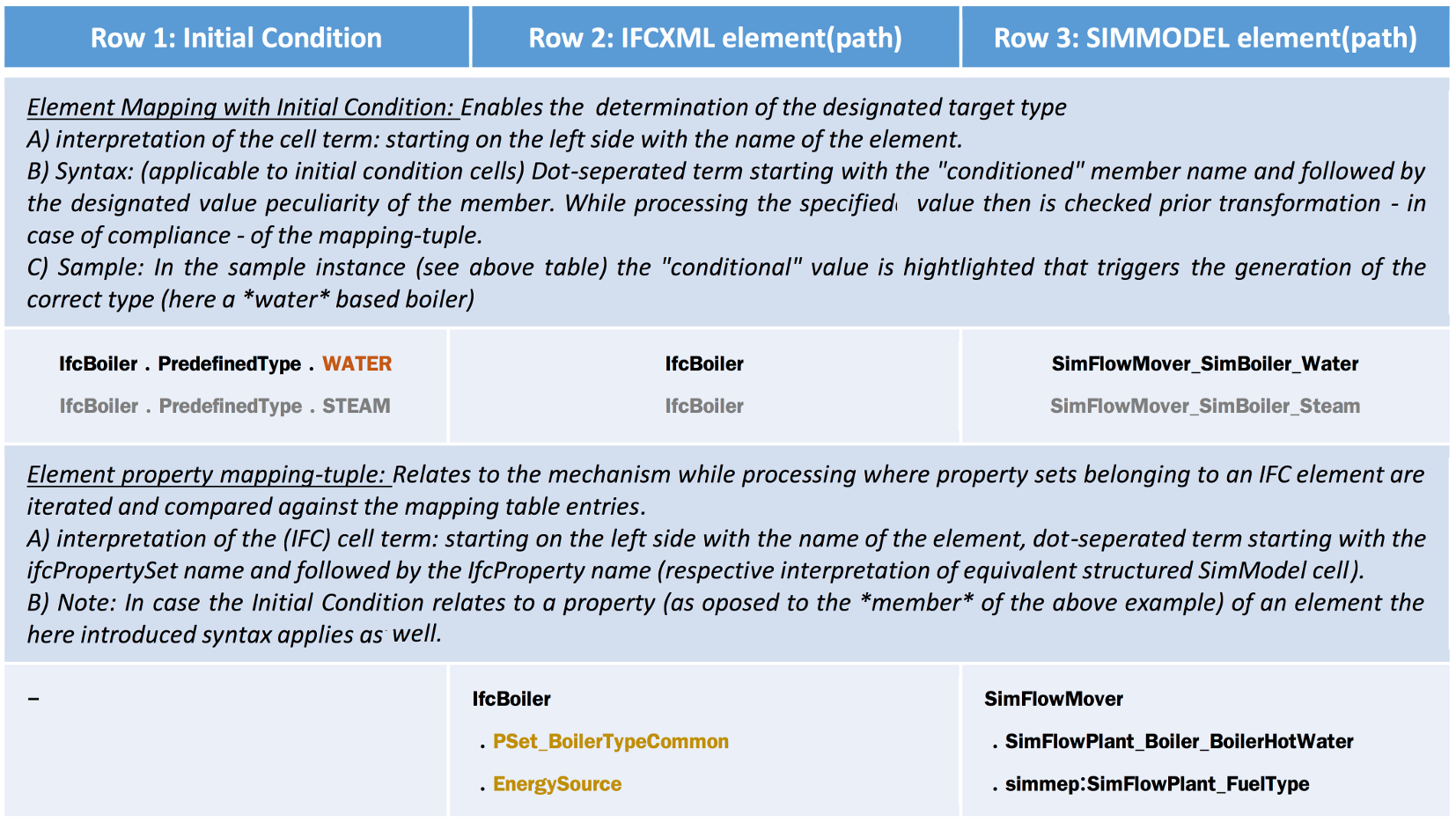
Fig. 7.20 Commented syntax example of the CSV mapping table
The simple “point-syntax” of the term further enables e.g. the specification of mappings between nested elements, and completes the machine readable mapping concept. Based on this mapping syntax definition and without having the mapping table fully formulated in detail, a (dynamic) requirement basis for the implementation of the designated conversion tool is given.
7.4.3.4.4. Implementation
For realizing the converter with XSLT 1.0, the above introduced concept blocks one, two and four were integrated into an XSLT transformation procedure which is described in the third concept block. Fig. 7.21 shows the overall procedure where the green templates - ifcXML root element and Production Templates for respective IFC elements - realize the overarching main procedure.
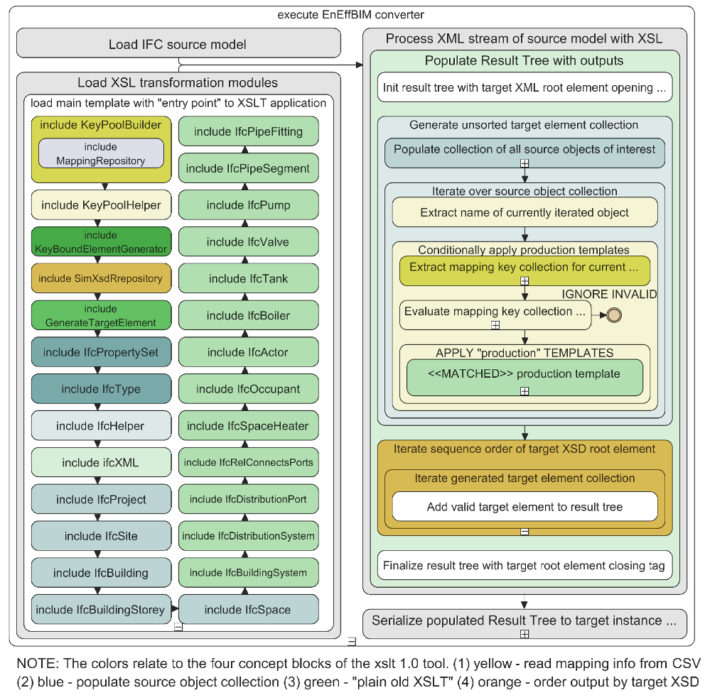
Fig. 7.21 Recursively superimposed concept blocks of final tool specification
Thereby recursively nested templates of the first (blue) and second (yellow) concept block extend the static procedure with mechanisms to
- a priori collect all relevant IFC entities from the source model stream and
- inject the conversion instructions from a CSV table that is delivered by the BIM*Q platform.
Fig. 7.21 depicts the generation of the target root element “SimModel”. Within the green box “MATCHED production templates” a recursive sub-procedure handles the generation of the target elements and their content. For further reading we refer to [EvB16]. In summary, a demand-led, dynamic and scalable solution was realized. Future developments (or other configurations) are supported by providing the full implementation of the tool as open source (access via https://download.building-lifecycle-management.de).
7.4.4. libSimModel C++ library
This section describes the transformation system developed for linking BIM with different Modelica libraries. In the system, SimModel acts as the BIM container to save BIM data generated from IFC, for example, HVAC, geometry, property data of HVAC systems and equipment, simulation configurations, etc.
7.4.4.1. SimXML Data Binding and Syntax Validation
The data file of SimModel is an XML-based file named SimXML. It saves all the SimModel data as a structured XML document that is in accordance with the syntax defined by the SimModel schema. Thus, this sub-section introduces the XML data binding technique for accessing SimXML and validating its syntax. XML data binding is the process of extracting data from a structure representation of XML documents and presenting it as a hierarchy of objects that correspond to a document vocabulary. This allows us to manipulate SimXML data in a more direct and efficient way. We selected the open source, cross-platform CodeSythesis XSD [Cod14] as our system XML binding parser. It is an efficient framework whose parser can be adjusted for custom applications. The automated XML data binding of CodeSythesis XSD will generate a C++ API for accessing the data stored in SimXML after parsing the SimModel schema. For the SimModel schema version 2.2, 2611 C++ classes representing different SimModel objects are generated for the data manipulation in a given SimXML file. The XML syntax validation performs a number of checks on the XML document to prevent the construction of an inconsistent object model, such as an object model with missing required attributes or elements. Our SimXML validation relies on the underlying Xerces-C++ XML parser embed in CodeSythesis XSD. It checks the SimXML data against the given SimModel schema, and outputs the errors found into a log file. The syntax validation is enabled by default and is very useful during the development stage to detect problems with the data model at an early stage. For a user of the framework, this validation does not play a significant role anymore, since the changes to the SimModel model are finalized.
7.4.4.2. SimModel Hierarchy Parsing and Visualization
A model hierarchy is an arrangement of the model elements, e.g., objects, names, values, categories, etc., in which the elements are represented as being “above,” “below,” or “at the same level as” one another. Consequently, the SimModel consists of a hierarchical tree structure saving such relationships between different SimModel data elements (see Fig. 7.22).
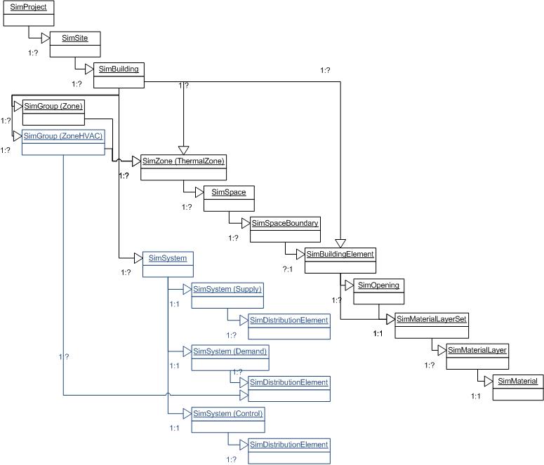
Fig. 7.22 SimModel hierarchy tree structure.
As illustrated in Fig. 7.22, a SimProject class object is normally the root node of this hierarchy tree representing a unique simulation project. This root node can store multiple links that refer to different building design alternatives. Each design alternative also refers to a set of building elements, zones, HVAC systems distributed inside the building, etc. Therefore, the SimModel hierarchy saves a set of different SimModel elements as well as the links between them in a tree-based structure. At the bottom of the SimSystem sub-tree, different types of SimDistributionElement nodes are created to save different HVAC components located at different sides of the SimSystem, e.g., a hot water boiler will be saved as a child SimDistributionElement node of the SimSystem water supply side. At each SimDistributionElement node, a list of child nodes are created for saving different physical connections between these HVAC components, e.g., the pipe connections within a hot water looping system for connecting the boiler and pump. The physical connections saved by these child nodes represent the SimModel topology.
In SimXML, each model element is given a unique long type ID that distinguishes it from all other elements. Each parent element of the SimModel hierarchy links to a child element by saving its ID. As a result, “parse SimModel hierarchy” is a recursive algorithm that detects each SimModel element, locates its position in the hierarchical tree and creates a tree node with a link to its data. After that, we can also recursively iterate each node of this hierarchy, retrieve the link to the SimXML data element and print out the element data for visualizing the created hierarchy.
7.4.4.3. SimModel to Modelica Mapping Rule Schema and Rule Filter
The mapping rule concept was first introduced in mathematics, representing a particular transformation. This transformation describes the conversion of a source model data into a target model data under the constraints specified by a given equation system. As SimModel is significantly different from the data model of a specific Modelica library [CMO+14], e.g., AixLib or BuildingSystems, we also need to define a set of mapping rules that can handle the difference between these two different data models. [WCR+15][WMO+14] proposed a set of different mapping rules that can convert the SimModel data into the Modelica model data defined by a specific BPS library AixLib [EBC14]. Based on this work, we developed a mapping rule schema in XML Schema Definition (XSD), containing the data model of the mapping rules between SimModel and different Modelica libraries [CWT+15]. We can thus efficiently re-use this mapping rule schema, originally developed for our transformation system, to define different sets of mapping rule instances for different target Modelica libraries. Mapping rules are classified according to three different levels in the schema:
- The first level is library mapping, which is designed to link different mapping rule instances for different Modelica libraries.
- The second level is component mapping, which is responsible for mapping SimModel components, e.g., a boiler of the HVAC system, into the corresponding component of the Modelica library specified by the first level mapping.
- The third level deals with the internal properties mapping of the components defined by the upper-level mapping rules.
Czarnecki and Helsen [CH06][CH03] discussed fundamental work on data model transformation. In context of their work we can view transforming SimModel data model to Modelica code as a special case of model-to-model transformations. We only need to provide the meta-models for the source model and the target programming language as well as the transformation defined with respect to the meta-models. A transformation engine transfers the source model data into the target programming language model. In our case, the source model is SimModel and the target language is Modelica. The transformation is an instance of the mapping rule schema saved as XML file format and the transformation engine contains a set of filters translating the model data by filtering the mapping rule instance. The source model data is stored in SimXML file and the target programming language model is the Modelica code, based on a specific BPS library.
7.4.4.4. SimModel Python API for Modelica Code Generation
The main parts of the transformation system are implemented in the C++ programming language, in order to satisfy the requirements of model transformation speed and the access to low-level system features, such as virtual memory allocation. Script programming languages, like Python, are heavily used for pre- and post-processing of Modelica. They are more flexible and easier to use for controlling the procedure of Modelica code generation based on techniques like pre-defined code templates and interpretation engines. Therefore, this sub-section introduces a generic API developed for interfacing SimModel C++ library and the script programming language Python, in order to better control the Modelica code generation by separating the translation logic from code generation.
We developed our prototype for this generic API based on a technique named language binding. In computer science, a binding from a programming language to a library is an API providing the glue code to use that library in a particular programming language. In the context of our generic API, bindings are wrapper libraries that bridge the C++ and Python programming languages in order to re-use the SimModel API generated for C++ in Python.
According to the testing on different binding libraries, e.g., ctypes, Cython, Boost.Python, we use SWIG [SWI15] as the binding libraries to wrap the SimModel API for data access out of Python. Compared to other binding libraries, SWIG is easier to port the interface of a large C/C++ library to other languages, like Python. It is an open-source and battle-tested binding software used by large companies, e.g., Google. It keeps both the C++ and Python code clean, i.e. not altering Python itself such as Cython is doing. SWIG provides C++ compatible data types, and allows calling functions in the Dynamic Link Library (DLL) or the other types of shared libraries from Python. In the system prototype, we exposed the mapped or translated SimModel components and their internal properties into a Python-based Modelica code generator via the SWIG wrapper. In order to provide Python with full controls on SimModel internal data, we also exposed more data objects from the SimModel hierarchy as well as the topology into Python via the generic API. Fig. 7.22 illustrates SimModel hierarchy exposed for Python.
7.4.5. Mapping Rules
Several steps need to be considered to complete the mapping between the SimModel data model and the Modelica libraries. Fig. 7.23 and Fig. 7.24 shows two BPMN (Business Process Model and Notation) process diagrams to illustrate the decisions and steps needed for a successful mapping.
As indicated in Section 7.3.7, in the formal mapping process we distinguish between object and parameter mapping.
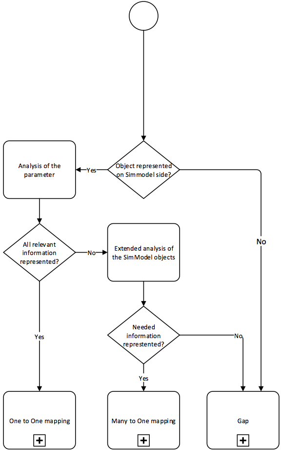
Fig. 7.23 BPMN process diagram for the object mapping
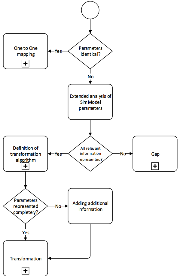
Fig. 7.24 BPMN process diagram for the parameter mapping
The object mapping is performed as a first step in order to find all the relevant objects to represent the data needed in the specific Modelica library. Fig. 7.23 shows the sequence of the object mapping. Checking if the object needed for Modelica is represented in the SimModel data schema is the first step. To understand the objects of each side, the SimModel and the Modelica library documentations should be considered. If an object is not defined in SimModel, either the missing object needs to be added to the existing data schema or the Gap mapping rule needs to be applied. If it is represented, the next step is to check if all parameters in the SimModel object are sufficient for the targeted Modelica object. One to One mapping can be applied, if all relevant data are available. If further information are needed, other SimModel objects need to be considered in addition. In case several objects are needed to provide the relevant information, the Many to One mapping rule defines those. If still some information is lacking, the data schema of SimModel needs to be extended again by applying the Gap rule.
Fig. 7.24 illustrates the next steps to complete the mapping between the SimModel data schema and the Modelica libraries. If the parameters on both sides are defined identically, a simple One to One mapping rule can be applied. If additional information is needed, further parameters should be considered. Several SimModel parameters can be combined to define a single parameter on the Modelica side. To perform a combination of parameters, the transformation mapping rule needs to be applied. For defining the transformation algorithm, it can be necessary to add external data.
A specific example of the transformation rule is demonstrated below. The value of the set temperature for a gas boiler on the SimModel side is defined using the unit Celsius, whereas the unit for the Modelica side needs to be defined in Kelvin.
The transformation algorithm for this mapping process is
where \(a\) is the temperature setpoint of a gas boiler in the SimModel data model.
As shown, the algorithm transforms the set temperature from Celsius to Kelvin, adding 273.15. Thus, the SimModel value is transformed and describes the relevant data for the Modelica side.
7.4.6. Python Tools for Modelica Code Generation
Python as an interpreted language is used widely in the Modelica community for scripting, workflow automation, pre- and post-processing and as a glue language. Using the wrapper for the libSimModel library generated by SWIG, most functions from the C++ library can be called from Python. The Python tools using the libSimModel API so far are a Qt based viewer and editor for the SimModel object tree, a high-level API that adds further functionality and implements the topology mapping and the code templating tool CoTeTo, that is used for generating Modelica code.
7.4.6.1. SimModelTreeView
Based on the API generated by SWIG, a simple viewer for the SimModel object tree has been implemented as a PyQt widget. It uses QTreeView and reads data from the API on demand when unfolding the tree. A second widget is implemented for viewing and editing the attributes of objects. Both widgets can be called on their own or be embedded in another GUI or be imported as a module.
7.4.6.2. High-Level API
The API as generated by SWIG reflects the functions defined in C++. For user convenience, a set of Python classes that can be loaded as a module has been implemented on top of that API. A UML diagram for these classes is shown in Fig. 7.25.
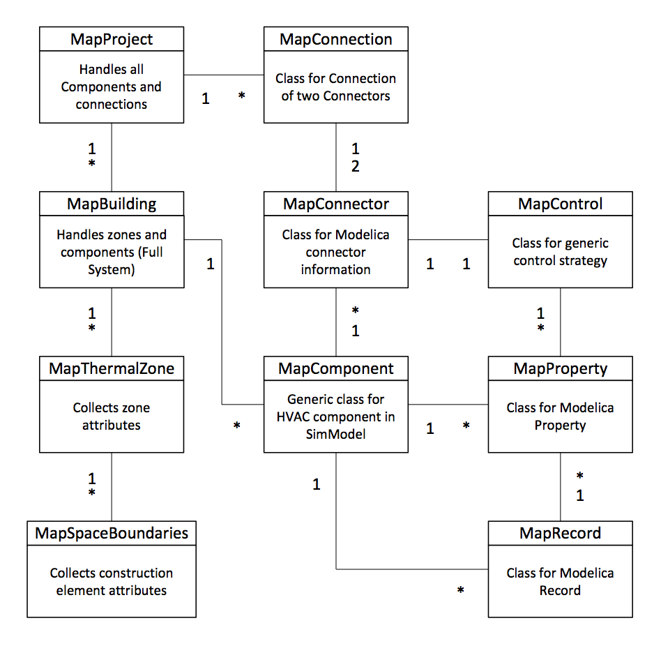
Fig. 7.25 UML diagram for the high-level API.
The classes each have attributes that are accessible using the dot notation. One attribute is, where applicable, an iterable list of child objects. The Python classes as well implement the topology mapping which is described in the following paragraph.
7.4.6.3. CoTeTo: Code Templating Tool
The actual Modelica code generation is implemented as a tool named CoTeTo, which stands for Code Templating Tool [TRR+15]. Although designed for this project, this tool was implemented in a way that it can be used standalone and in other software environments. CoTeTo is released under the MIT open-source license at https://github.com/UdK-VPT/CoTeTo .
In this project, Modelica models for a set of different model libraries have to be generated using a common data source. Each library needs separate filtering and output of data because of different modeling approaches. These libraries are currently under development and are likely to change in the future as well. This requires a flexible and generic data conversion framework to allow for future changes. Thus, the framework should allow flexible output components for different libraries in multiple versions as well as flexible input components, both should be easy to maintain even for non-programmers.
The workflow of CoTeTo and the coupling to other tools within the toolchain is shown in Fig. 7.16.
We designed CoTeTo to be used by graphical, command line and library level interfaces. The multiple access possibilities open the framework to be used by a larger community.
The fact that Python does not require extensive compilation cycles helps with rapid development. The following section will give an overview of the components and their functionality. We divided CoTeTo into input components (Data APIs) and output components (Generators). A Generator depends on a specific Data API (defined by its name and version).
7.4.6.3.1. The Template Approach
There are two general concepts for the generation of textual output within a computer program.
One approach is to embed print()-statements for text strings and data in the structure of a program.
This is useful for nearly static, well-defined structures of the data set and of the textual output.
The other approach is template-based, where placeholders for the content are embedded in a text file (a template for the output). Besides placeholders templates also offer control structures. Thus, template-based model generation allows complying with fixed Modelica language syntax and adding flexible model content in the same file. One advantage is the flexibility for the end user, who does not necessarily need to dive into the programs’ internal structure, but can enrich the template file with placeholders and simple programming constructs, whenever the used Modelica models change. This workflow is much like the form letter function in office software, which fills some variable address fields in a text document from a database.
The template approach fits well into the flexible structure of the CoTeTo framework, as it is independently usable for different information sources. From the list of available template engines Mako [Bay14] and Jinja2 [Ron14] seem to fit best into CoTeTo. At this point support for both is implemented.
7.4.6.3.2. Input - Data APIs
A Data API is a Python module that defines a prescribed way to fetch data sets from a data source. Although we use the Python language to write the CoTeTo, Data API functions can interface with other languages.
Different Data APIs and different versions can be used in parallel. Sample modules for reading JSON, XML and CSV files exist in CoTeTo. This allows flexible processes during development and testing. There is no definition for the structure of the returned data items, since different data sources contain different types of data (tree, table, graph, map). It is the job of the corresponding output Generator to understand the data delivered by the related Data API.
The most important Data API in the Annex 60 context is the interface to the C++ library libSimModel, which handles the SimModel parsing and the mapping to Modelica. Seen from the Python framework and from CoTeTo it defines the data source used to fill the placeholders in the output templates.
7.4.6.3.3. Output - Generators
Once all relevant data have been loaded into CoTeTo, it is passed to the output component, called Generator. We designed the Generator to contain all items needed to generate the code for a specific Modelica library. This includes
- filter functions,
- the meta model structure,
- text templates,
- additional configuration and information and
- additional files.
The filter functions, meta model structure and text templates are used and applied by CoTeTo. Additional files like the mapping rules XML file can be stored inside the Generator.
Some data need manipulation that may not fit well into the mapping rule mechanism. For this purpose, Generators can include filter functions (Python code) that we call between the data API and the templates. The filters are custom-built to the used library. In our case, they may include simplification of geometric relationships and calculation of model specific parameters. Another application of filters would be the creation of annotations for the graphical appearance and placement of model components in the Modelica code.
One major challenge in the automated generation of Modelica models is the flexibility of Modelica. Generally said, setting up useful models needs the knowledge of an experienced user. We are following the approach to encapsulate this knowledge in library specific meta-models and templates. One essential task is the appropriate connection of components. The API returns the connection information corresponding to the SimModel ontology, which differs from the one in a Modelica library. The meta model checks if the connection is applicable, if not, it manipulates it.
The text templates are the last step in the process chain. The template engine combines the data structures returned by the Data API and possibly manipulated by filters with the text templates to files with valid Modelica code. The templates in a Generator can be split into several files to ease maintenance.
Generators can be easily exchanged between different installations, as they are simple folders or even zip-files with a defined structure. Generators can be maintained and edited with standard system tools like a file manager and a text editor. Creating a new Generator is as simple as copying a folder with an existing Generator and changing the name or version number in a text file.
One example for a Generator template using Mako template engine is given in following listing. Static elements can easily be implemented as plain text in the template (e.g. within line 1). A Dollar symbol, followed by curly brackets mark the placeholder, e.g. MapData.used_library in line 1 is replaced by the Python class attribute used_library in the complied template. Control elements, like for loops, are identified by a percentage symbol and follow the Python syntax, with the exception that indentation is not supported and the control element has to be closed (e.g. %endfor, line 6). This example template generates a simple model, by printing the library location (target_location) and individual name (target_name) in the first loop from line 4 to 6 and their corresponding connections in line 9 to 13.
1 2 3 4 5 6 7 8 9 10 11 12 13 14 15 | within ${MapData.used_library};
model ${MapData.name}
%for comp in MapData.hvac_components:
${comp.target_location} ${comp.target_name}();
%endfor
equation
%for con in MapData.connections:
connect(
${con.con_a.parent.target_name}.${con.con_a.name},
${con.con_a.parent.target_name}.${con.con_a.name});
%endfor
end ${MapData.name};
|
7.4.6.3.4. User Interface and Handling
There are currently three ways to use CoTeTo:
- CoTeTo can be imported in Python software as a module library. CoTeTo works both with Python 2.7 and 3.3+. All functions are usable via the modules API.
- A command line interface can be used interactively or called from other software. It allows listing the available Data APIs and Generators and executing a Generator with a data source URI to produce the text output.
- The graphical user interface (GUI) is implemented using PyQt4. It allows flexible browsing and editing of all components and included files and the execution of selected Generators. The GUI can be used as a standalone tool (see Fig. 7.26) or embedded in PyQt4-based applications as a widget.
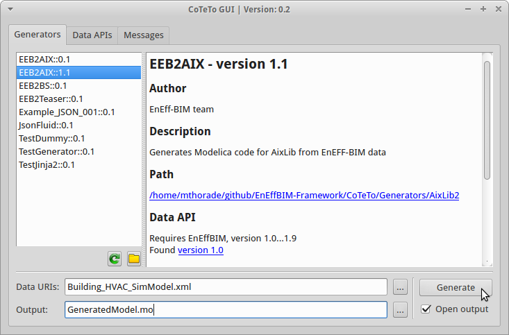
Fig. 7.26 Screenshot of the CoTeTo user interface
7.4.7. Topology Mapping
As already stated in the introduction of this section, the Mapping Rules (Section 7.4.5) deal with objects and parameters from SimModel to a specific Modelica library. In addition to the Mapping Rules in its current status we need information about model topology (e.g. number, type and name of Modelica connectors attached to the model) to generate valid Modelica models.
We define model topology as the way that the model in a certain object oriented language or information model is described in terms of connection to other models. In addition it offers the possibility to characterize which parts of the model are included in the object and which additional objects need to be connected in order to work appropriate (e.g. different control elements). This topology differs from SimModel to Modelica libraries. One advantage of the presented work is that the transformation process complies and adapts with the BIM and the specific model topology in Modelica libraries. Neither the topology of the BIM model nor the topology of the Modelica library need to be changed.
Furthermore the topology of models in different Modelica libraries may differ, even if the models describe the same behavior/object. To extend the information provided by the BIM with these Modelica and library specific information we developed a set of Python classes. This section describes the different topologies of SimModel and Modelica in more detail, taken the AixLib as an example. Furthermore, the Python classes and the usage for other libraries are demonstrated.
In SimModel as well as in Modelica different objects are connected by connections with different connectors. However, the type of connections differs for these languages. For the given use cases and with a special focus on BPS we identified four connector types in Modelica to be significantly more important. Table 7.2 lists these Modelica and the corresponding SimModel connector types. In addition, Fig. 7.27 show the different connectors in Modelica, the left column shows the connectors dedicated for design input, the right for design output respectively. However, for Fluid and thermal connectors this is just a guideline as these connectors are acausal. The Fluid connector can be used for various media (e.g. water or air) by changing the Medium attribute inside the connector.
Fig. 7.27 Different connector types in Modelica (graphical representation).
| MSL | SimModel |
|---|---|
| Fluid connector (Medium: water) | Water connector (cold, hot) |
| Fluid connector (Medium: air) | Air connector |
| Thermal connector | Air connector |
| Real connector | Control connector |
| Boolean connector | Control connector |
As Table 7.2 shows one connector type in Modelica may correspond to several connector types in SimModel and vice versa. The topology mapping needs to consider the different connectors and in the code generation distinguish between them. This may be done by setting the correct parameters in the model, for example in the case of a water connection in SimModel, the corresponding media of the fluid is also set to water, by an mechanism in the Python topology classes.
Not only the type of connections differs from SimModel to Modelica but also the number of connectors per specific model and in particular the function and name of the connectors can differ from library to library (e.g. in the case of different Pumps). Thus, it has an effect on the topology of the models in this library and the library itself. As the transformation process was designed to be flexible enough, the library developers do not have to change their library, but adapt the transformation process. This is advantageous as the library can be developed for different purposes, without delimiting the development because of BIM required restrictions. Other pre- and post-processing tools of the individual library do not need to be changed.
In the following we present three examples and compare the topology and connections of the Modelica objects from AixLib (the topology may differ in other libraries) and SimModel. The considered objects are:
- Pump
- Radiator in a thermal zone
- Temperature controlled valve
7.4.7.1. Pump
The first example considers a pump. In SimModel the specific object is called SimFlowMover_Pump_VariableSpeedReturn. It has three different connector types:
- SimNode_HotWaterFlowPort_Water_In
- SimNode_HotWaterFlowPort_Water_Out
- SimNode_DigitalControl_HWLoop_DigitalSignal_In
Fig. 7.28 Connector types in Simergy shown on a pump (graphical representation)
Water_In and Water_Out illustrate the causal approach of SimModel and are used to connect the pump within a hydraulic loop. The DigitalControl input is used to attach a certain control object to the model. The AixLib holds five different implementations that could be used as a pump. We take AixLib.Fluid.Movers.Pump, which is AixLib specific, and AixLib.Fluid.Movers.FlowControlled_dp, which is inherited from an Annex60 library example to point out differences (see Fig. 7.29). Both models have two Fluid connectors to connect them within a hydraulic loop. This concept aligns with the topology in SimModel. Further, both Modelica models have inputs to control the pump. AixLib.Fluid.Movers.FlowControlled_dp uses a real input named dp_in to imprint the pressure difference of the pump, which may come from arbitrary control strategies. In contrast to that the developers of AixLib.Fluid.Movers.Pump implemented a control strategy in the model itself, to use the model for specific applications. The control strategy uses a boolean signal to switch between two different operational characteristics. This input is called IsNight. Both the type and the name of all three connectors need to be added within the topology mapping. In addition, the control strategies of the pumps need additional model objects (e.g. a boolean pulse), the instantiation and correct connection of these additional objects can also be assured in the topology mapping.
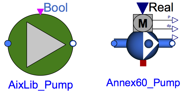
Fig. 7.29 Comparison between AixLib.Fluid.Movers.Pump and AixLib.Fluid.Movers.FlowControlled_dp
7.4.7.2. Radiator in a Thermal Zone
To distribute thermal energy into a thermal zone, radiators can be used. The integration into a hydraulic loop is very similar to the procedure described in the above example and thus not part of this section. To semantically connect a radiator and the thermal zone, the concepts of SimModel and the approach used in AixLib differ, see Fig. 7.30. In SimModel the radiator is attached (by referencing it with an ID) to a ZoneHvacGroup, which is a collection of all HVAC equipment used or aligned to that certain zone. In AixLib the distribution of thermal energy is done by thermal connectors, that calculate the heat flux for convective and radiative heat transfer respectively. Therefore both, the radiator and the thermal zone hold each two thermal connectors. Between these connectors the topology mapping needs to instantiate the correct connections [connect(Radiator.heatPortCon, ThermalZone.internalGainsConv) and connect(Radiator.heatPortRad, ThermalZone.internalGainsRad)]. It is worthwhile mentioning that the names of the connectors and models are again model and library specific. Further standardization would simplify the conversion process in the future.
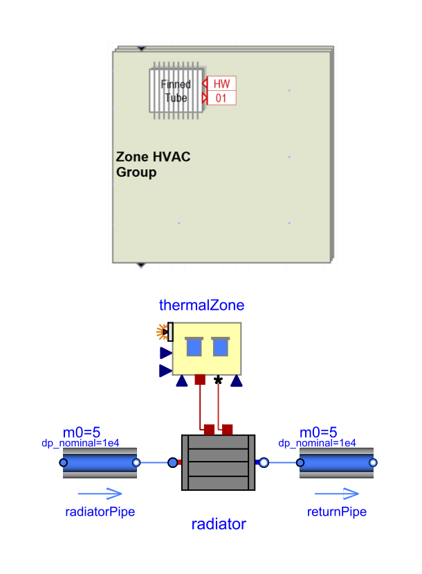
Fig. 7.30 Connection between a radiator and a thermal zone in SimModel and AixLib
7.4.7.3. Temperature Controlled Valve
This example illustrates the different handling of controls in SimModel and AixLib. We consider a PID controlled valve for flow regulation in a hydraulic loop. The measured variable in this case is the air temperature in the thermal zone, set point is a constant value and the manipulated variable is the opening of the valve. SimModel has no such control, the radiator is controlled by an ideal controller that is connected with SimNode_DigitalControl_HWLoop_DigitalSignal connectors to the thermal zone and the ZoneHvacGroup, respectively. For AixLib we need to instantiate a PID controller, a constant block and a temperature sensor (see Fig. 7.31, all taken from MSL) and connect them in the correct manner with the valve and the thermal zone air node.
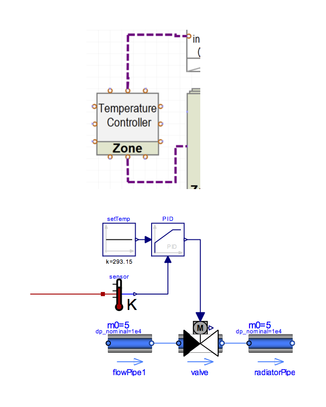
Fig. 7.31 Temperature controlled valve in SimModel and AixLib.
7.4.7.4. Python Classes for Topology Mapping
The set of python classes used for topology mapping can be obtained from Fig. 7.32. The idea is to provide highly reusable classes with general functions for the transformation of SimModel and Modelica, including the processing of data from libSimModel API and providing functions for topology mapping. Individual library can directly use the classes (e.g. MapProject or MapBuilding) or inherit them and extend it with library specific information (e.g. MapThermalZone and MapComponent). The Python classes and an example implementation for the AixLib models can be found at https://github.com/EnEff-BIM/EnEffBIM-Framework.
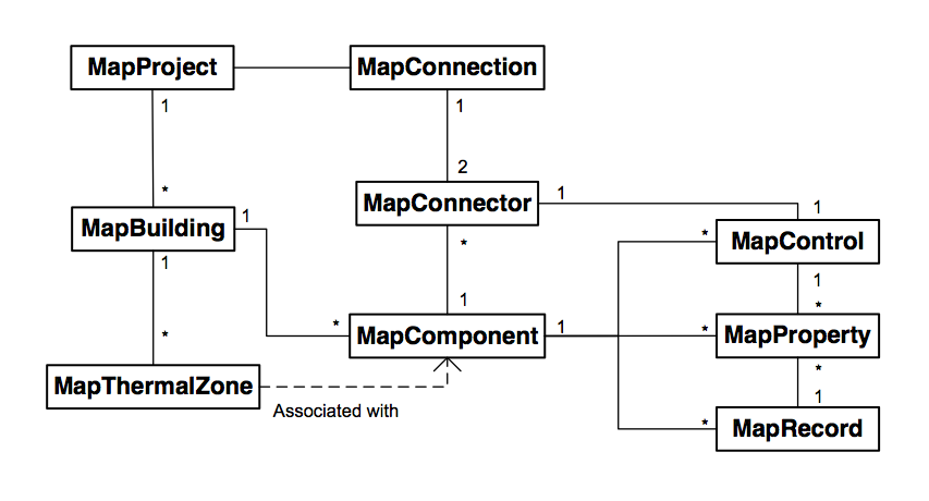
Fig. 7.32 Simplified UML diagram of the Python classes used for applying information from libSimModel API and topology mapping.
7.5. Use Cases and Demonstration
To test the tool chain and to analyze the different data models, in the Annex 60, a set of nine use cases was defined. Each use case is applied in the different steps of the tool chain. By modeling each of these use cases in IFC, SimXML and Modelica each (where possible, see more at the end of this section) it was possible to compare data structures and to determine requirements for the transformation from BIM to Modelica. While the information structure in IFC and SimModel will not change, the structure of Modelica libraries differs, as already described. Table 7.3 provides an overview of the use cases. All use cases contain different HVAC-systems, to ensure that different components with multiple model topologies are considered. For the sake of better readability, this list does not include other necessary components like pipes, ducts, pumps or control elements, however, these components are part of the use cases as well.
| Identifier and name: | HVAC System (generation + distribution) |
|---|---|
| 1.1 Boiler | gas boiler + radiator |
| 1.2 Boiler | gas boiler, buffer storage for domestic hot water + radiator |
| 2.1 Heat Pump | heat pump, buffer storage + radiator |
| 2.2 Heat Pump | heat pump + floor heating |
| 3 CHP | combined heat and power unit + radiator |
| 4.1 AHU | air handling unit heating |
| 4.2 AHU | air handling unit cooling |
| 5 Multi Zone | combination (Boiler 1.1, AHU 4.1, AHU 4.2) |
| 6 Rooftop Building | test case for geometry processing |
The transformation of BIM to Modelica in this project focusses on HVAC components. Thus, we use the same thermal zone for the first seven use cases to calculate the thermal losses. This test room is parameterized according to German guideline VDI 6007-1 (Fig. 7.33). Basic characteristics of the room are:
- One room with a window, on the second floor of a three story-building
- Floor area: 17.5 m²
- Outer wall area: 3.5 m²
- Window area: 7 m²
- Adiabatic (no heat transfer through) internal walls and slabs. Heat transfer only through the outer wall and the window
- internal loads: occupancy, plug loads, lighting
- Weather-data: TRY dataset for Germany, zone 5 (Aachen)
Fig. 7.33 The single room architecture for the use cases 1.1 - 4.2.
For weather boundary conditions we are using a Test Reference Year (TRY) from Aachen, Germany. Internal loads for persons, plug loads and lights are taken from DIN 18599 and SIA 2024.
Use case eight was defined as multi-zone test case. Use case nine is dedicated to geometry processing and testing.
7.5.1. Use Case 1.1: Boiler with Radiator
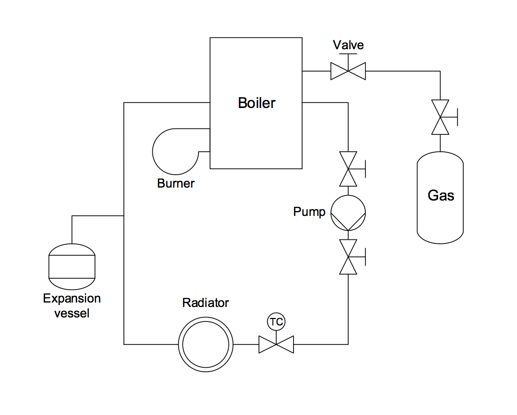
Fig. 7.34 Use case 1.1.
Short identification
HVAC-system of Use Case 1.1 (Fig. 7.34) consists of the following items:
- gas fired boiler
- pump
- expansion vessel
- radiator with P-controlled valve
- pipes to connect components
Gas fired boiler
The gas boiler has a maximum heat output of 1300 W. The flow temperature is set to a constant value of 340 K. The volume of the water inside the heat exchanger is 0.01 m³. The efficiency is indicated in the form of Table Table 7.4 as function of part load ration.
| Part load ratio | Efficiency |
|---|---|
| 0.0 | 0.78 |
| 0.2 | 0.78 |
| 0.4 | 0.82 |
| 0.6 | 0.84 |
| 0.8 | 0.86 |
| 1.0 | 0.88 |
Pump with night set back
The pump has a maximum head of 5 m and a maximum flow of 3 \({m}^3/h\) (if the control strategy requires a maximum flow). The flow characteristics of the pump are given in Table 7.5 as dependence of the flow (in \({m}^3/h\)). During 6 pm and 5 am the night signal is turned on and the minimal characteristics are used.
| Flow [\({m}^3/h\)] | min head [m] | max head [m] |
|---|---|---|
| 0.0 | 0.6 | 5.0 |
| 0.5 | 0.4 | 4.5 |
| 0.75 | 0.3 | 3.0 |
| 1.3 | 0.0 | 2.5 |
| 1.5 | 0.0 | 1.5 |
| 2.5 | 0.0 | 1.0 |
| 3.0 | 0.0 | 0.5 |
| 3.5 | 0.0 | 0.0 |
Radiator
The radiator type is a single-row radiator with one convector and cladding. The characteristics of the radiator can be taken out of Table 7.6. These characteristics follow the description of the European standard ISO EN 442 .
| Parameter | Value |
|---|---|
| Nominal power | 979 W |
| Nominal flow Temperature | 75 °C |
| Nominal return Temperature | 65 °C |
| Nominal room Temperature | 20 °C |
| Volume | 3.15 l |
| Mass of steel | 19.58 kg |
| Percent of radiative heat | 0.35 |
| length | 1 m |
| height | 0.6 m |
| Exponent for heat transfer | 0.35 |
Control valve of radiator
The valve is connected to a P-Controller. The gain is 0.1, lower and upper limits are 0 and 1, respectively. The set temperature for the controller is set to 20 °C.
Pipes
All pipes used to connect components have the same properties. They are 3 m long, have a diameter of 0.03 m and a roughness of \(2 * {10}^-5 m\) .
Expansion vessel
The expansion vessel ensures a constant pressure of 1 bar on the suction side of the pump.
7.5.2. Use Case 1.2: Boiler with Radiator and Domestic Hot Water
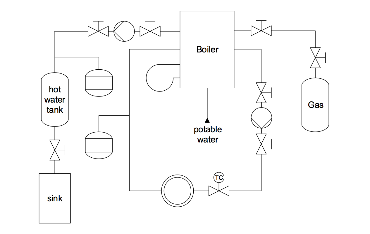
Fig. 7.35 Use case 1.2.
Short identification
HVAC-system of use case 1.2 (Fig. 7.35) consists of following items:
- gas fired boiler (see Section 7.5.1)
- pump (see Section 7.5.1)
- expansion vessel (see Section 7.5.1)
- buffer storage for domestic hot water
- three way valve for switching loading/unloading of buffer storage
- radiator with P-controlled valve (see Section 7.5.1)
- pipes to connect components (see Section 7.5.1)
Gas fired boiler
The domestic hot water system and the water for the heating system is seperated. The potable water has a seperate port connected to the public water system.
Hot water tank
The hot water tank is only used for domestic hot water. The usage of domestic hot water is triggered by a simple time table to indicate when hot water is used. The set value of the flow temperature is 70 °C. The buffer storage has following parameters:
| Parameter | Value |
|---|---|
| diameter | 0.72 m |
| storage height | 1 m |
| volume of heat exchanger inside storage | 0.05 m³ |
| heat exchanger heat transfer coefficient | 1500 W/(m² K) |
| heat exchanger area | 20 m² |
| thermal conductivity of insulation | 0.04 W/(m K) |
| thickness of insulation | 0.2 m |
| internal heat transfer coefficient | 1500 W/(m² K) |
| external heat transfer coefficient | 15 W/(m² K) |
Three way valve
The three way valve is used to control loading of the buffer storage, with a simple on/off strategy. The storage is supplied with hot water (valve fully opened) when the room temperature is warm enough and the temperature on the top level of the storage is too cold. In any case the valve opening to the buffer storage is set to zero.
7.5.3. Use Case 2.1: Heat Pump with Radiator
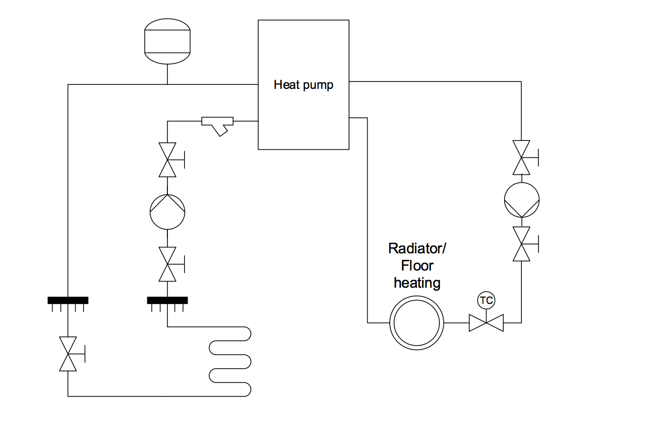
Fig. 7.36 Use case 2.1 & 2.2.
Short identification
HVAC-system of use case 2.1 (Fig. 7.36) consists of following items:
- heat pump with fixed source temperature
- pump (see Section 7.5.1)
- expansion vessel (see Section 7.5.1)
- radiator with P-controlled valve (see Section 7.5.1)
- pipes to connect components (see Section 7.5.1)
Heat pump
The heat pump characteristics are given in Table 7.8 and Table 7.9. Based on these tables the electric power and the heat flows of the condenser can be calculated as a function of source and sink temperatures.
| Sink/source temp. [K] | 273.15 | 283.15 | 288.15 |
|---|---|---|---|
| 308.15 | 203 W | 212 W | 217 W |
| 328.15 | 295 W | 323 W | 337 W |
| Sink/source temp. [K] | 273.15 | 283.15 | 288.15 |
|---|---|---|---|
| 308.15 | 885 W | 1162 W | 1300 W |
| 328.15 | 811 W | 1060 W | 1185 W |
7.5.4. Use Case 2.2: Heat Pump with Underfloor Heating
Short identification
For this use case the thermal zone is slightly changed. Instead of a radiator for heat distribution into the thermal zone an underfloor heating system is used (Fig. 7.36).
HVAC-system of use case 2.2 consists of following items:
- heat pump with fixed source temperature (See Section 7.5.3)
- pump (See Section 7.5.1)
- expansion vessel (See Section 7.5.1)
- underfloor heating
- pipes to connect components (See Section 7.5.1)
Underfloor heating
The underfloor heating is installed for the whole area (17.5 m²) of the obtained room. Further characteristics are described in Table 7.10.
| Parameter | Value |
|---|---|
| Pipe spacing | 0.2 m |
| external diameter of pipe | 0.02 m |
| thickness of pipe | 0.0025 m |
| thermal conductivity of pipe | 0.35 W/(m K) |
| thickness of concrete above pipe | 0.02 m |
| thickness of concrete below pipe | 0.02 m |
| thermal conductivity of concrete | 0.35 W/(m K) |
| density of concrete | 0.35 kg/m³ |
7.5.5. Use Case 3: Combined Heat and Power (CHP) Unit
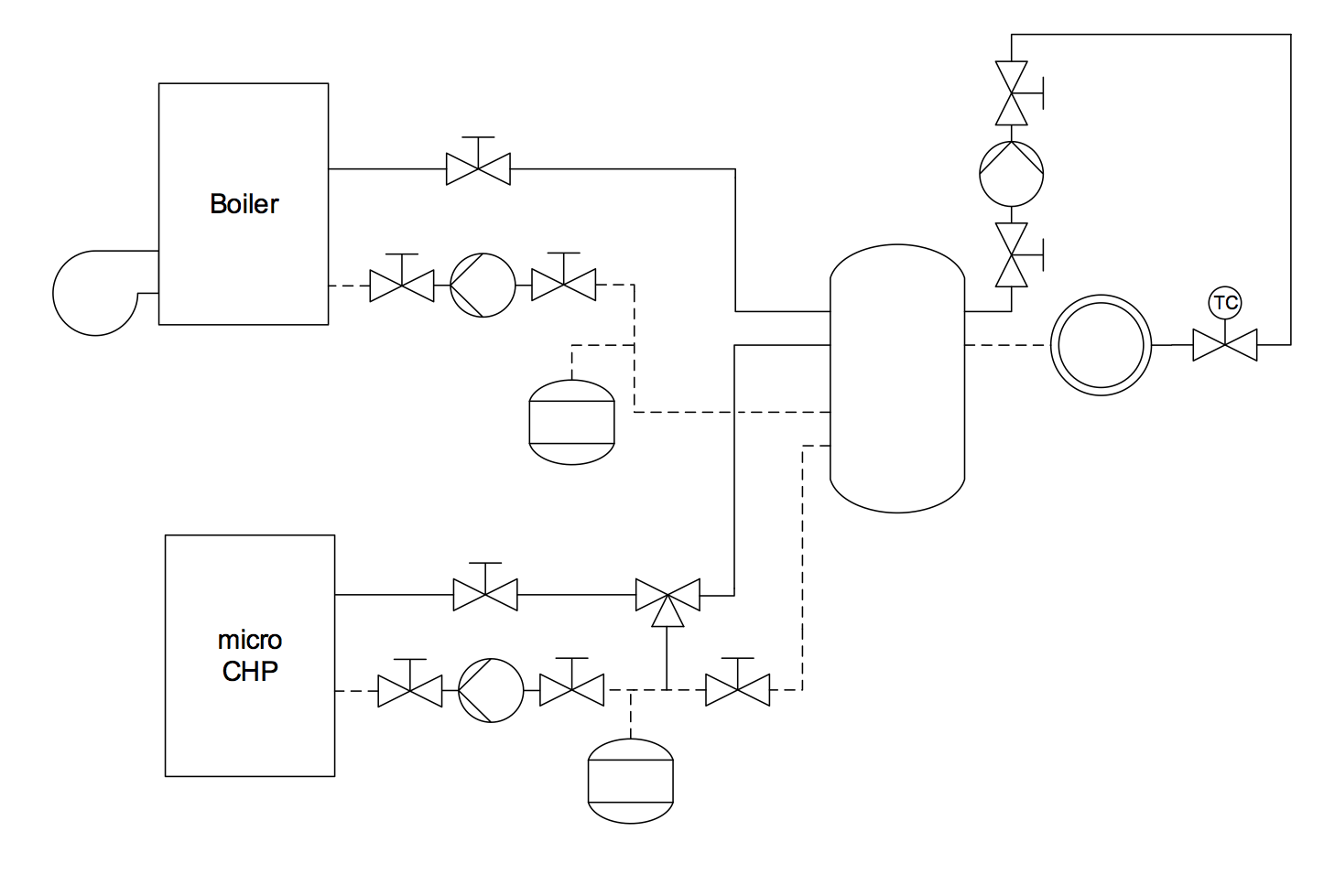
Fig. 7.37 Use case 3.
Short identification
HVAC-system of use case 3 (Fig. 7.37) consists of following items:
- CHP unit
- pump (See Section 7.5.1)
- expansion vessel (See Section 7.5.1)
- radiator with P-controlled valve (See Section 7.5.1)
- pipes to connect components (See Section 7.5.1)
- buffer storage (See Section 7.5.2)
- three way valve for loading and unloading
Combined Heat and Power unit
The boiler is replaced by a Combined Heat and Power unit with following characteristics:
| Parameter | Value |
|---|---|
| Electrical output | 1000 W |
| Thermal output | 2500 W |
| Electrical efficiency | 0.27 |
| Thermal efficiency | 0.67 |
| Fuel utilization rate | 0.92 |
| Modularity | 0.5 - 1.0 |
Three way valve
The three way valve is used to control unloading and loading of the buffer storage. If the thermal zone requires thermal energy, first the buffer storage is completely unloaded, until it is not able to satisfy the flow temperature. The storage is loaded if the temperature in the thermal zone is above the set temperature and the buffer storage temperature reached the flow temperature plus a additional temperature difference of 5 K.
7.5.6. Use Case 4.1: Air handling Unit for Heating (AHU Heating)
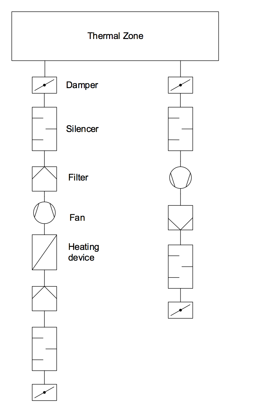
Fig. 7.38 Use case 4.1.
Short identification
HVAC-system of use case 4.1 (Fig. 7.38) consists of following items:
- Air ducts
- supply/ return air damper
- silencer
- pressure controlled fans for supply/ return air (radial/ axial)
- air filter for supply/ return
- electric device for heating
Damper
The dampers for supply and exhaust air are set to a constant opening fraction of 0.7. The face area of the dampers are 0.1 m².
Fan
The fan is pressure controlled to supply the zone with heated air. The pressure difference is controlled with a PID-Controller PID (gain = 100, time constant integrator = 20 s, time constant deriative = 4 s). Lower and upper limits for pressure difference are set to 18 Pa and 550 Pa, respectively. The heat added by the fan is negligible.
Filter, silencers, ducts
Several components like the filter, the silencer or the ducts introduce pressure losses into the system. These pressure losses are combined and set to 300 Pa.
Heater
The heater increases the supply air temperature to reach the room set temperature (20 °C). The maximum temperature of the supply air is set to 40 °C. The power of the heater is set 1300 W and controlled with a P-Controller, the pressure loss is 200 Pa.
7.5.7. Use Case 4.2: Air Handling Unit for Cooling (AHU Cooling)
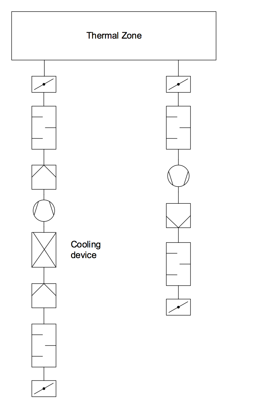
Fig. 7.39 Use case 4.2.
Short identification
HVAC-system of use case 4.2 (Fig. 7.39) consists of following items:
- Air ducts (see Section 7.5.6)
- supply/ return air damper (see Section 7.5.6)
- silencer (see Section 7.5.6)
- pressure controlled fans for supply/ return air (radial/ axial) (see Section 7.5.6)
- air filter for supply/ return (see Section 7.5.6)
- Evaporative, adiabatic cooling device
Evaporative, adiabatic cooling device
The cooler reduces the supply air temperature to reach the rooms set temperature, by adding moisture the air stream. The temperature of water that is added to the fluid stream is set to 8 °C. The added water is controlled with a P-controller using the zone set temperature of 20 °C.
7.5.8. Use Case 5: Multi Zone Model
Short identification
This case study building represents a three story office building, located in Aachen.
Fig. 7.40 Case study building, address: Mathieustraße 30, 52074 Aachen, Germany.
The building primarily comprises office spaces but also contains kitchens, washrooms, corridors, mechanical rooms and a server room. The heating system consists of a gas boiler and radiators (see Section 7.5.1). The BIM model developed in Revit Architecture is shown on the right and a picture of the building is shown on the left of Fig. 7.40. The heating systems, also modelled with revit is shown in Fig. 7.41
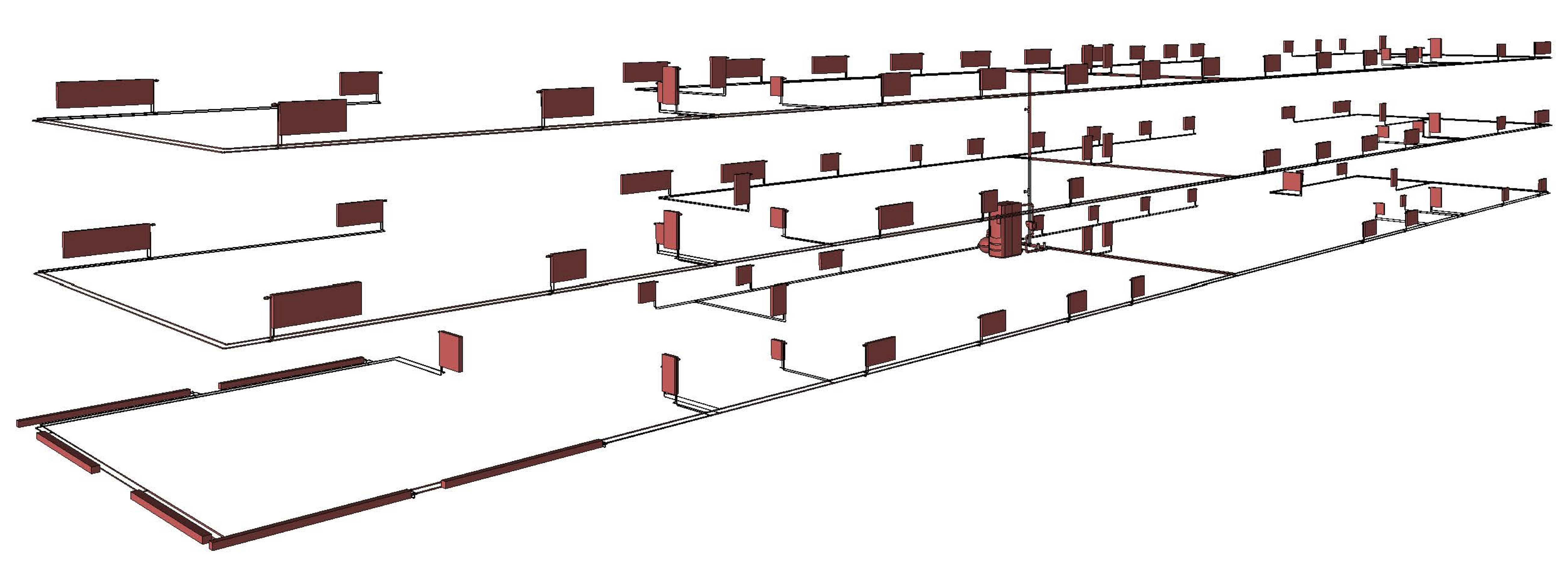
Fig. 7.41 Whole heating system of use case five, modelled with Revit 2016.
The thermal zones are defined, according to the DIN V 18599. It defines the thermal conditions for the room type. The office type rooms should have an air temperature of 21°C. The presence of persons is between 7:00 and 17:30. The metabolic rate is equal to a sitting person, emitting 80 Watt per square meter skin surface. The light switches on at 17:00 and other equipment, like computers and screens are activated the whole time people are present. Because the offices are heading in different directions the operations of the zones to guarantee the thermal comfort is different. One side of the building is heading mostly to to the west and the other side is heading mostly to the east. The differences in the solar radiation requires different operations for the heating systems. The corridor should have an air temperature of at least 15°C and the light is turned on at 16:30. Nearly no solar radiation hits the corridor directly. The different thermal zones are shown in Fig. 7.42, differently coloured.
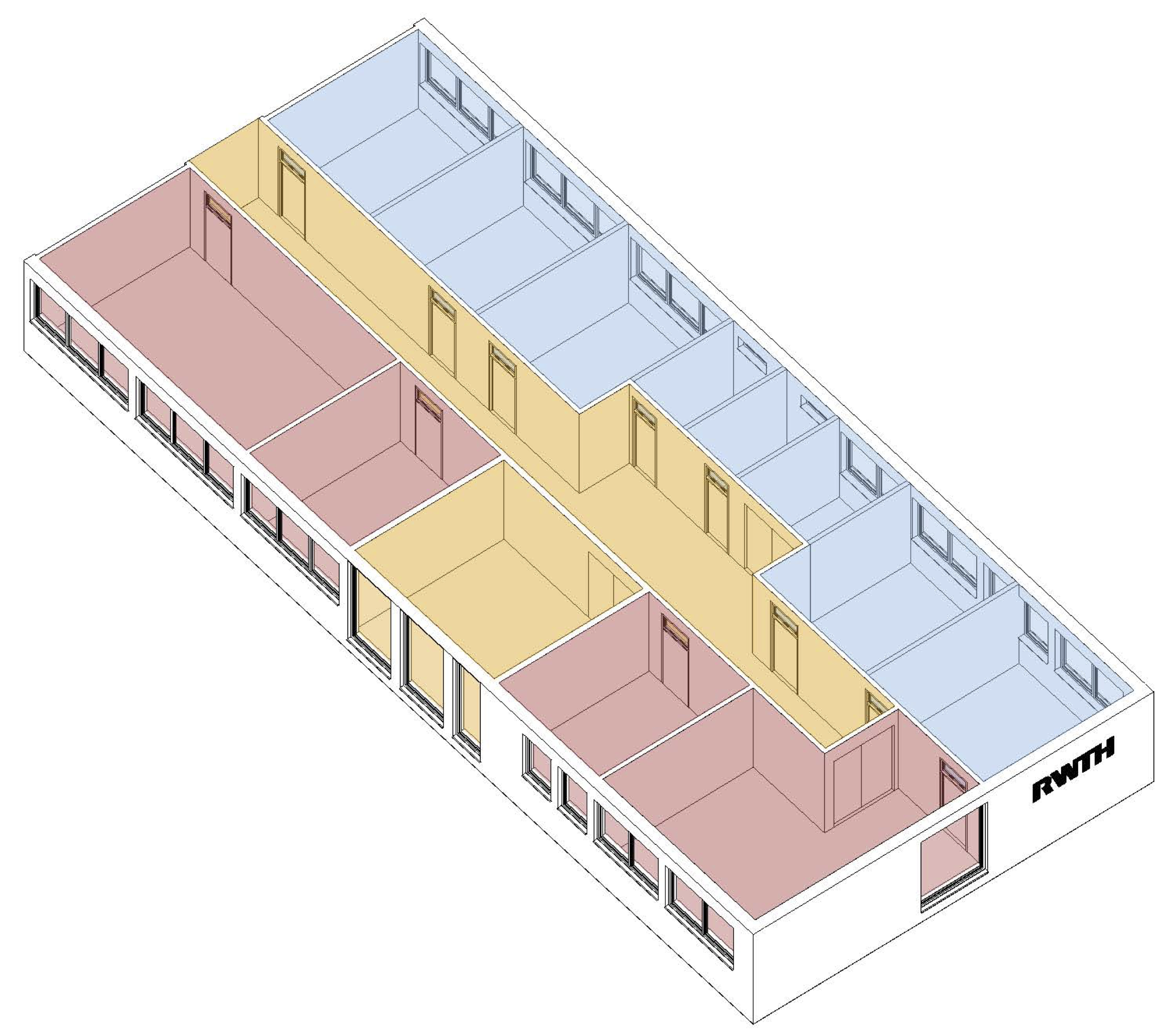
Fig. 7.42 Thermal zones for the western and eastern offices and for the corridor, defined in Revit 2016.
| Parameter | Value |
|---|---|
| Thermal zones | 2 on each floor |
| Thermal output | 80490 W |
| Pump performance | 9068 Pa |
| Volume flow | 2.22 l/s |
| Number of radiators | 96 |
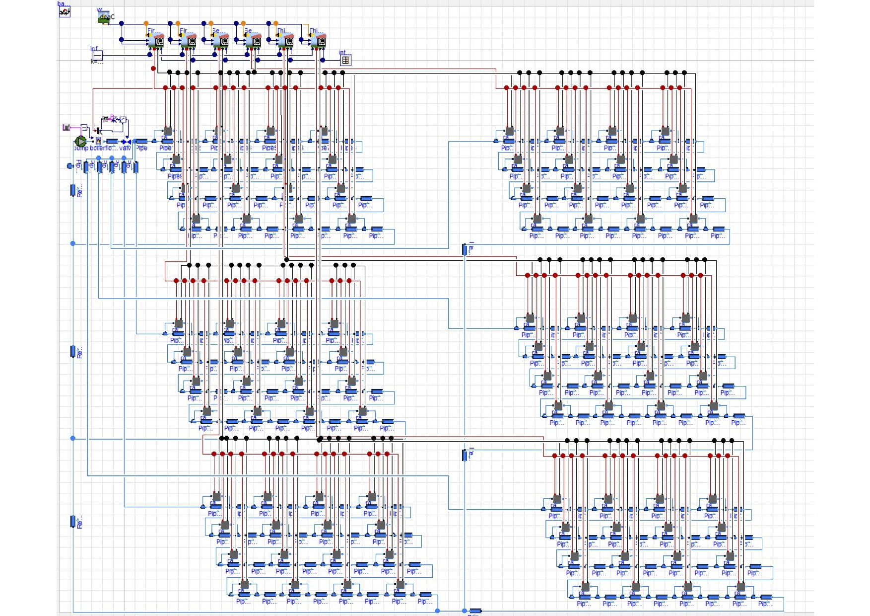
Fig. 7.43 Use Case 5 modeled with the AixLib Modelica library.
Use Case 5 modeled in Modelica, using the AixLib library is shown in Fig. 7.40. The six thermal zones are represented on the top. To improve the simulation performance, the thermal zones were simplified in an additional step. The nine thermal zones have been comprised to six thermal zones. The corridor is separated, so that one half of the corridors’s thermal zone is part of the eastern and the other part belongs to the western thermal zone. The heating system is modeled below the zones. All 96 radiators are represented, to serve the building.
7.5.9. Use Case 6: Rooftop Building
Building geometry modeling for use with Modelica algorithms must be precise and must include all relevant detail, must be “clean” (i.e. error-free) and must be thoroughly checked and validated. If not, Modelica algorithms can lose their effectiveness. As virtually all major model-based CAD tools have the ability to generate building geometry models that are precise, it is always the modeler’s task to create models precise enough to meet the geometry definition needs of Modelica algorithms, and to assure that these models are technically error-free and verifiable [BMNG16]. Technically error-free models do not contain modeling errors and pass all tests with model checking tools. An example of such a model checker 3D view after successful validation is shown in Fig. 7.44. Yet, such models may still not be verifiable because buildings data used in the modeling process may be incorrect. Even the most competent modeler cannot create an error-free and verifiable model without access to trustworthy data about the building.
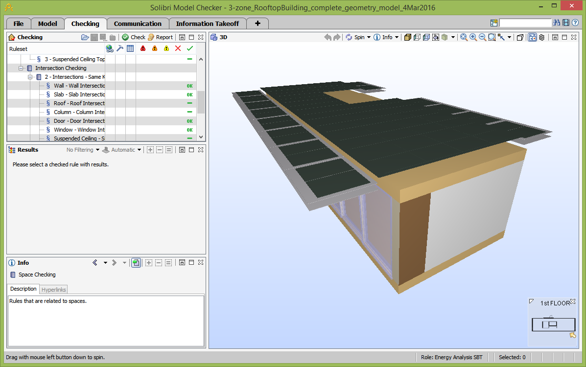
Fig. 7.44 Geometry model of the Rooftop building in Solibri Model Checker.
In the cases of modeling existing buildings, ideally the modeler has access to “as-built” documentation that provides reliable data about building construction. Unfortunately, “as-built” documentation seldom defines what was actually built – it does not document last-moment construction and installation changes. This inevitably results in “as-built” model inaccuracies, which contribute to the gap between simulated and measured building performance.
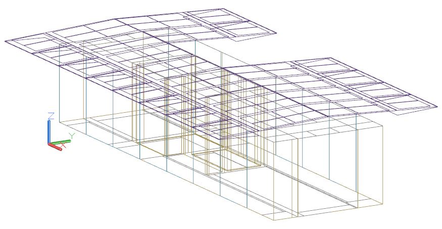
Fig. 7.45 Geometry model of the Rooftop building in passive state as imported into EnergyPlus, showing space boundaries, PV panels and shutters in their original position.

Fig. 7.46 Computer generated perspective image of the Rooftop building placed in Berlin city-scape (source [GFMAE14]).
The Rooftop Building is a good example of “best-practices” modeling for BEP simulation (Fig. 7.45). Its geometry model was built specifically to provide precise geometry data for use in the execution of Modelica algorithms that model energy systems installed in the building. As shown in Fig. 7.45, the building features an elaborate system of fixed and movable PV panels; panels directly above the building are fixed, while those projecting over the building sides are movable to optimize solar incidence angles during the day, as well as provide needed shading and shuttering. The building was an entry in the Solar Decathlon Europe 2014 [UBTB14]. The Decathlon entry was as well documented as one can expect at the end of design. Yet, some of the critical modeling data are missing in the documentation; other critical data contradict each other.
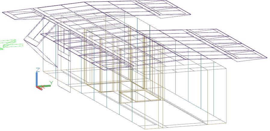
Fig. 7.47 Orthogonal projection of the Rooftop building’s geometry model in active state as imported into EnergyPlus, reflecting PV and shutter positioning shown in Fig. 7.46.
Fig. 7.46 is a computer generated “artist’s view” of the building, copied from the project documentation. Fig. 7.47 shows the building geometry model, generated using best available information from the same project documentation that mimics the positioning of movable PV panels and shutter shown in Fig. 7.46. The modeler had to improvise and guess some of the missing information and, in the case of conflicting data, to subjectively decide which data to use. Visual comparison of Fig. 7.46 and Fig. 7.47 shows what was expected (Fig. 7.46) and want appears to have been built (Fig. 7.47). Finally the resulting Modelica model is shown in Fig. 7.48. Fortunately, the Rooftop Building is being reconstructed and instrumented at the UDK- Berlin campus. This is providing a unique opportunity to record true “as-built” data, re-model the building geometry and see how closely simulation results can match energy performance measurements in the building.
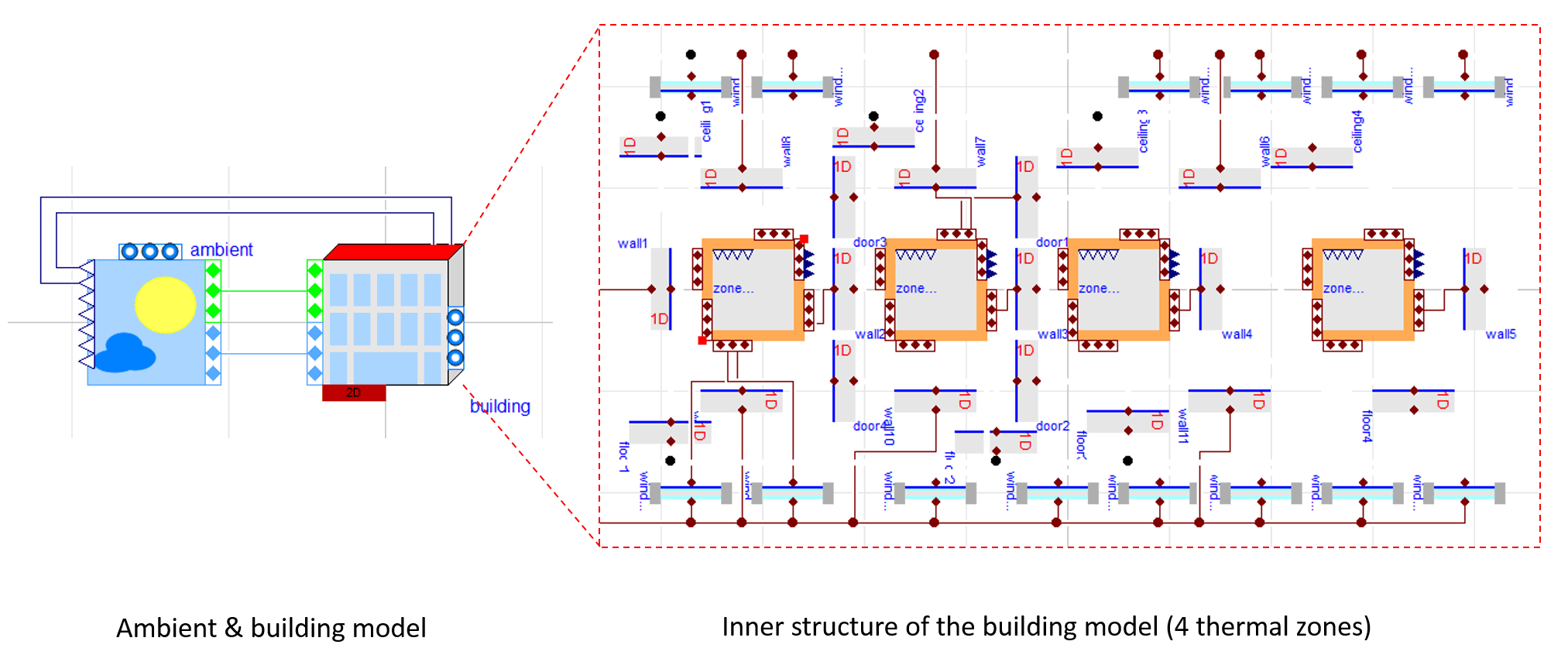
Fig. 7.48 Screenshot of the Modelica model of the roof top building.
7.6. Limitations of the Framework and Future Work
This subchapter describes the limitations of the framework focusing on generic limitations rather then today’s technical limitations which are improving over time. Furthermore, we discuss future work that is enabled by this development.
7.6.1. Limitations
The basic limitations of this framework or tool chain lies in the fact that various data models and tools are used. The tool chain is restricted to the functionality of each tool and data model. For example, HVAC components that are not available in Modelica libraries reduce the list of supported components. The same is true if any other tool or data model is not supporting a particular HVAC object. The distributed development in small tools also makes changes that influence multiple tools time consuming and sometimes difficult. E.g., changing a parameter in SimModel does create the need for updated mapping rules from IFC to SimModel as well as from SimModel to Modelica. In that context, the implementation of control objects turned out to be quite cumbersome since no tools exist that define controls and have a relevant IFC export and/or import functionality. In this area we developed a so-called workaround and attach relevant properties to the object that is controlled. This was necessary since controller objects are not available in the MEP CAD applications. One of the biggest challenges in this subtask was the flexible nature of Modelica and its libraries as well as their continuous development. While significant progress towards a standardized Modelica library development has been made through the Annex 60 base library, there still exists potential to standardize more aspects of the Modelica libraries. From a data model and mapping perspective additional standardization and library creator agreements would simplify future mapping and conversion efforts. E.g., currently connector names of components can be any arbitrary string. Yet another limitation is the quality of BIMs. While model checking tools exist and are further developed, the understanding of providing data models of high quality is not present in practice yet. Another aspect is that the generated Modelica models are just a starting point and need further fine tuning at the instance level of the Modelica models.
7.6.2. Future Work
While the developed tool chain is limited in scope and is a first prototype, the following developments could be based on it:
- Further specification of the MVD to include further relevant HVAC components
- Officially certified MVD that is implemented by various software applications.
- Extensions of the IFC data model for missing concepts that we identified within this project (see Section 7.3.5.3)
- Further development of the prototype tools to cover more HVAC components.
- Further development of the Modelica libraries to include missing components.
In order to allow for international collaboration and further developments, all in this project developed code and models related to the transformation process are made available as open source. The Annex 60 framework therefore provides a solid and well-documented base for further developments.