10. Activity 2.2: Design of District Energy Systems

10.1. Introduction

Recent developments to reduce the energy use of buildings focus on the integration of renewables and on energy efficiency. European legislation enforces that by 2020 all new buildings are nearly Zero-Energy Buildings (ZEBs) and it requires the deployment of a European Smart Grid. The shift in the energy infrastructure leads to new requirements and technical challenges as the interaction of buildings becomes increasingly important. To quantify the required interaction among buildings and the grid, as well as the restrictions caused by the existing neighborhood topologies and grid configurations, an integrated modeling environment is needed. This activity focuses on the use, verification and demonstration of Modelica libraries from Activity 1.1 and co-simulation tools for multi-scale simulation from Activity 1.2 to assess District Energy Systems (DES). The focus of this activity extends the traditional focus on individual building performance to DES. The analysis of these systems requires an integrated simulation platform that is capable of simulating simultaneously the energy demand of multiple buildings, the thermal and electrical energy distribution grids and the control systems.

The work that was carried out in this activity consisted of three main parts:

1. A literature study focusing on the modeling of DES
2. The development of a common exercise to model DES within Modelica environments
3. The use of co-simulation techniques to model DES

Section 10.2 presents a description of the main components typically found in DES. Section 10.3 addresses the modeling of multi-scale energy flows in districts and presents an overview of simulation tools and environments to model these systems. The overview discusses both Modelica and non-Modelica implementations. Section 10.4 reports on the common exercise that has been set up to analyze the capabilities of the current Modelica libraries of the Annex 60 participants and provides a first step to develop a comparative model validation test for district energy simulations: a DESTEST. In this exercise, a relevant simulation case (including building definition, occupant behavior, grid definition etc.) is developed for two purposes. Firstly, the set can be used to analyze relevant research problems such as how to design district heating systems and how to integrate renewables in districts. Secondly, the information and challenges gathered during the development will be used for setting up a framework to test District Energy System simulation tools. Although the simulation of DES within one software environment has many advantages and makes it a desired solution, scalability of the numerical methods to large models are still a challenge if one solver is used for the whole system of equations. Therefore, in Section 10.6, the opportunities and threads for co-simulation techniques related to DES simulation are analyzed. Finally, Section 10.7 presents conclusions and perspectives.

10.2. Description of District Energy Systems

A DES comprises all components that enable the delivery of energy services in a district. This typically includes electricity, gas, heat or cool, possibly at cascading temperature levels. However, in this section, modeling of gas networks are not discussed.

10.2.1. Electrical Versus Thermal Energy

Although the generation of electrical and thermal power have always been closely related, at least in power plants relying on combustion, their respective carrier grids have experienced a separate evolution. Fig. 10.1 shows an overview of commonly used technologies and their respective energy sources.

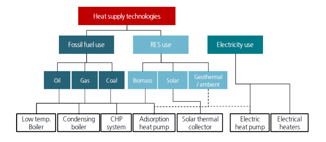
Fig. 10.1 Overview of heating technologies and their respective energy sources. Source [Com16b].

The International Energy Agency reports [Age14] that worldwide, electricity has the largest final energy consumption by far. Fig. 10.2 shows the produced and consumed annual electric energy and heat worldwide in 2014. However, note that a substantial part of electric energy is also used to meet heating and cooling demands by use of electric heaters and boilers, heat pumps and chillers. With a trend towards installation of more heat pumps, it can be expected that the electric energy fraction for the building sector will increase compared to the heat fraction.

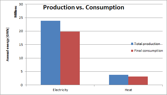
Fig. 10.2 Worldwide electricity and heat production and consumption in 2014. Source: [Age14]

The previous section considers all end uses of electricity and heat. When looking at the categories of energy use, it can be seen that both forms of energy have approximately the same fraction of energy use in buildings (considering residential and community and public services to correspond to the energy demand of buildings), as can be seen in Fig. 10.3.

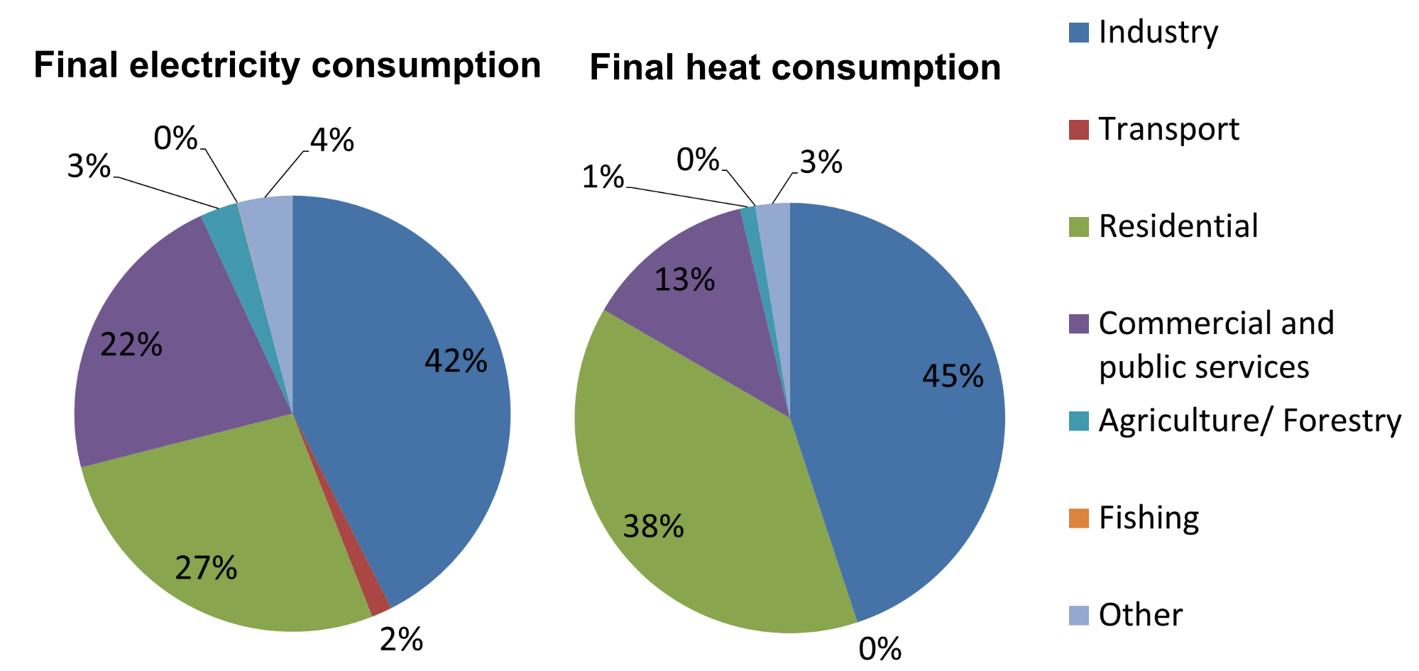
Fig. 10.3 End use fraction of electric and heat energy for different sectors in 2014. Source [Age14]

In the European Union in 2012, 50% of the primary energy use originated from building heating and cooling demand [Com16a], making it the largest energy sector. 18% of the primary energy comes from renewable energy sources. Biomass holds the largest share for heating only, namely 90% of renewable energy sources. [Com16b] further illustrates the end uses and sources of heating.

Part of this heating demand is provided through district heating and cooling networks. The share of district heating in the residential sector in the EU was 9% in 2012, and 8% for the industrial sector [Com16b]. For some EU countries, almost half of the national heat consumption is provided through district heating (Sweden, Denmark, Lithuania, Estonia and Finland).

On the other hand, district cooling systems are mostly used for office buildings. However, district cooling has not gained the same attention as district heating. This can be derived from the projected potential of both concepts in the EU Strategy for Heating and Cooling [Com16b] and the absence of district cooling in the Heat Roadmap for Europe 2050 [CNP13]. The installed capacity is less than 1% of that of district heating systems [Com16b].

There are more than 150,000 km of pipes in the district heating systems in the European Union [Com16b]. Denmark and Sweden have the most extended network, followed by Poland and Germany. However, the average system length varies greatly, signifying a large variation in the number of thermal networks in each country versus its size. Looking at the percentage of the population served by district heating systems, the lead is taken by Denmark and the Baltic states. On the other hand, the final energy use in district heating is by far, with twice as much energy as the runner-up, the largest in Germany. On a European average, almost half of the demand in district heating systems is met by dedicated boilers, while 42% comes from CHP installations. Only 5% is currently provided by directly recycling waste heat. Hence, the list of primary energy sources is still dominated by natural gas (40%) and coal (29%).

10.2.2. State-Of-The-Art in District Energy Networks

In the 1880s, the first district heating systems were installed, powered by steam [LWW+14]. In the meantime, district energy technology has evolved and matured. Three trends can be identified:

• a decreasing supply temperature for heating, and increasing supply temperature for cooling,
• a decreasing size and amount of material used for its components, and
• an increased share of standardization and prefabricated components.

Extending these evolutions, Lund et al. reason that after three generations of district heating systems, the next step must be the fourth generation with even lower heating supply temperatures and an increased focus towards the integration of renewable energy sources. Examples of mainly solar powered DES can be found a.o. in Canada (Drake Landing Solar Community [SMD+12]) and Denmark (Marstal district heating system [PS13])

The Swiss Competence Center for Energy Research is exploring an even further step forward with bi-directional thermal networks [SKS15]. Much like the electrical grid can convey energy both from a centralized generator to a consumer and back from a rooftop PV into the grid, a bi-directional thermal network uses a single circuit for both heating and cooling. When in net more cooling is needed than heating, the system circulates from a central plant in one direction. When more heating is needed, the system circulates in the opposite direction. In the case of a balanced system, no water flows through the central plant. Thus, in bi-directional systems, buildings can recover heat from each other directly.

Fig. 10.4 Bi-directional thermal network.

Fig. 10.4 shows an example schematic of a bi-directional thermal network. The plant guarantees that the hot side is kept between \(12^\circ \mathrm C\) to \(20^\circ \mathrm C\), while the cold side is kept between \(8^\circ \mathrm C\) to \(16^\circ \mathrm C\). The system uses near-ambient temperatures to maximize the efficiency of heat pumps. Unlike earlier generations of district heating, the bi-directional system need not be operated to serve the lowest and highest temperature needs. Rather, each individual building is equipped with heat pumps, allowing to locally boost the temperature up or down to the temperature required by the building. The system has the benefit of being modular extensible, allowing adding buildings, heat sources, heat sinks and storage without having to oversize the initial system.

Regarding electrical energy network at the district level, distributed generation by means of PV panels or micro CHP units is becoming more prevalent. However, in the low voltage grid, care must be taken that the voltage stays within an acceptable range. This becomes increasingly difficult with more distributed generation. On the other hand, electrical demand is also expected to go up in the very near future, with increasingly more air conditioning units, heat pumps and electric vehicles.

The integration of all these new technologies necessitate smart control strategies such as demand response, transactive controls or curtailing PV production in case of overproduction, in order to guarantee adequate system operation.

10.2.3. Components Typically Encountered in District Energy Systems

Next, we will describe the components that are typically encountered in thermal and electrical district energy systems

A general overview of thermal components typically encountered in district heating and cooling systems is given in [FW13]. Below, a short summary of components is provided. Models for these components must be available in a district energy simulation library.

Pipes:transport heat (or cold) from production sites to consumers in the grid. Substations:separate the primary (high pressure) network from the secondary (customer) side hydraulically. This is usually done by using heat exchangers to contain the consequence of leakages at the customer side. Control valves:regulate mass flows in different parts of the network. They regulate the flow that each customer receives and the bypass from the supply to the return pipe. The goal is to maintain the correct temperature in all parts of the network: high enough supply temperature, and a return temperature that is as low as possible [GW14]. Buffer tanks:store hot or chilled water for later use and hence limit peak power. Long term storage:  allows shifting energy for a long-time, usually seasonally. They include borehole fields or acquifers. Pumps and pressurization:  provide a pressure difference such that the water flows from the supply to the return side. For high temperature networks, they also prevent the water from boiling.

At the heat and cold production side, boilers, combined heat and power units, heat pumps or chillers are encountered. Furthermore, solar thermal boilers can be used to directly incorporate solar thermal energy.

For the simulation of electrical consumption in DES, typically only the low voltage grid is considered. Power from the high voltage grid is usually assumed to be available, but local power injection from decentralized production such as photovoltaics is possible. Hence, the components needed for electrical simulations are distribution lines (3-phases and neutral), transformers, power converters such as rectifiers, inverters and DC/DC converters, batteries, and PV panels.

10.2.4. Energy Demand

We will now characterize the thermal and electical energy demand.

The thermal energy demand consists of the demand for domestic hot water (DHW), space heating, process heat and cooling. The conditioning of indoor spaces can be provided with a large variety of systems, such as convectors, radiators, variable or constant air volume units, radiant ceilings and floors. The choice of the emission system determines the temperature at which the heat or cold is required.

The energy demand is largely determined by three aspects: the occupants, the weather conditions and the building characteristics.

Occupants influence the energy demand in the following ways:

• Desired temperature set point or comfort band in the heated and cooled spaces.
• Internal gains directly from occupants.
• Internal gains from appliances used by occupants (e.g., cooking, lighting, electronic devices).
• Domestic hot water demand.

These processes are characterized by high levels of uncertainty. One way to cope with this uncertainty is to model the energy demand stochastically. A software tool to calculate these uncertainties is presented by Baetens and Saelens [BS15].

The weather conditions outside of the modeled buildings determine the heating or cooling demand. Here, mostly solar irradiation and ambient temperatures are prevalent influence factors.

Related to this, the building characteristics such as the level of insulation, aspect ratio and building orientation determine how large the influence from the aforementioned weather conditions on the indoor climate is.

Electricity is needed for lighting and for powering home appliances. It can also be used to power thermal systems, such as heat pumps, cooling machines (air conditioning) or electric heating. Furthermore, electricity is needed to power pumps in the different parts of a thermal network and fans in the ventilation systems. Moreover, electrical cars cause an additional load but also an opportunity for electrical storage.

10.3. Modeling of District Heating and Cooling Systems

10.3.1. Introduction

DES models can be distinguished between physical domains, geographic scales and time scales.

Various modeling tools for DES exist. Many of the existing tools have limited support for modeling integrated energy systems. In tools that have detailed building and HVAC models, the study of electricity systems is idealized, often not allowing to assess the impact of renewable generation on the voltage stability. Other tools focus on medium or high voltage grids, but use simplified building and HVAC models for a very high number of households, sometimes not allowing to determine the required temperature levels.

Fig. 10.5 compares time scales and simulation objectives for district heating and cooling systems. Simulation can be used for time range of seconds for assessing water hammer effects to years for network design and investment planning.

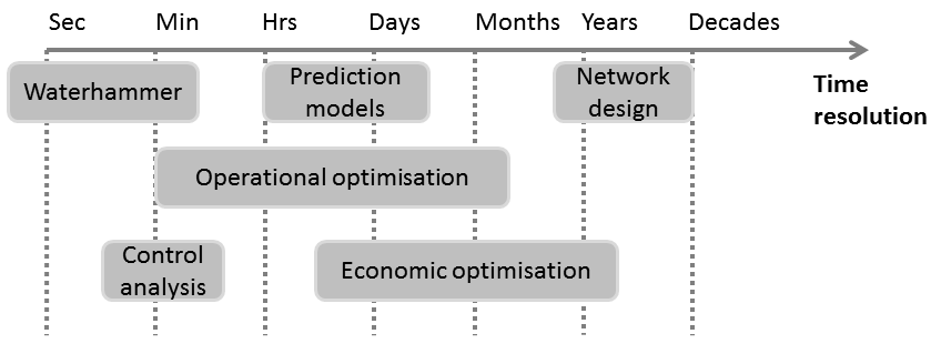
Fig. 10.5 Time considerations depending on the focus of the study.

10.3.2. Modeling Methodology

Modeling and simulation of district energy systems must cover different levels of detail and a large application range from components sizing to network topology design. In this section, a generic methodology for modeling a large scale system is presented in order to assess performances of DES, such as energy demand or efficiency as well as operational and control strategies. Three main steps can be highlight:

Grid and network modeling. The grid topology provided by the operator is aggregated and modeled into the simulation tool. The dynamic thermo-hydraulic behavior of a grid model is carried out with numerical models of the simplified and/or aggregated DES. Grid models include the implementation of the grid topology and pipe models.

Occupancy modeling. In the residential sector, customers needs consist of a combination of space heating or cooling, domestic hot water and electrical demand. Space heating or cooling can be based on models parametrized with physical properties of the buildings or regression functions on the basis of monitoring data. Electrical and domestic hot water demand are usually derived from statistical models.

More details on the determination of typical load profiles can be found in Section 10.2.4. Internal heat gains are deduced from occupancy profiles and activity probability functions. Process heat demand for industrial usage and/or for absorption chillers can be considered, but is not covered in this section.

Supply modeling. Heat plants and decentralized production are identified based on data provided by the grid operator and technical specifications. Operational strategies and control need to be implemented to balance energy and meet specifications.

Fig. 10.6 shows a schematic of all components to be modeled and how they interact.

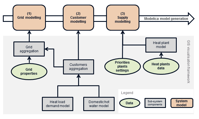
Fig. 10.6 Methodology flow diagram: example for a large district heating network

In order to facilitate both the process of modeling and the post-processing of simulation results, geographic information system (GIS) tools are commonly used. Detailed descriptions of the single components are reported in the following sections.

10.3.3. Data Acquisition

An increasing number of cities are creating 3D virtual city models for data integration, harmonisation, storage and visualization. Such an urban data model can provide a range of benefits as it can represent an information hub for advanced applications ranging from urban planning, noise mapping, augmented reality up to energy simulation. To this extent, CityGML is an international standard conceived specifically as information and data model for semantic city models at urban and territorial scale. It models principal urban features both geometrically and semantically, including buildings, land use, terrain and vegetation. For cities, a structured database for district energy system analysis should contain:

1. district network information such as topology, pipes characteristics, storage and production specifications,
2. building attributes such as building id, address, type (e.g. single family house), use, year of construction, year of refurbishment and total heated floor area.

Relevant parameters therefore can be extracted from the city model and aggregated to construct a district energy model.

10.3.4. Problems and Challenges

As part of any modeling work, challenges and problems might be encountered in the whole process, from the digitalization to the final assessment of network performance. The following list is the result of an Annex 60 survey in terms of problems encountered from the participants in their activities.

One of the main interests in modeling district heating networks is to simulate the rate of energy transport through the system. This transport is not only dependent on the water flow through the system, but also on the temperature levels in the network. Variations in temperature in a district heating system are mostly due to three phenomena [Pal00]:

• Changes in supply temperature, controlled by a system operator. These variations can be large and fast.
• Return temperature changes due to heat or cold transfer at customer substations. These variations are usually rather slow, but fast variations due to domestic hot water preparation are possible.
• Heat transfer between the pipes and their environment.

Temperature drops due to heat loss or infiltration in pipes are quite stable. However, the changes in supply and return temperatures affect the transient heat losses and the heat storage in the pipes. Heat losses represent the main source of energy losses in high temperature district heating systems. For the latest generation of district heating systems, due to the low supply temperatures, friction losses gain an increasing importance in the overall energy losses [LS12].

There is an important difference between flow and temperature dynamics [FW13]. Changes in the flow are quickly transferred to the whole network in form of pressure waves, typically in matter of seconds. Changes in temperature, however, are transferred relatively slowly, in relation to changes in the flow. Thus, the response time from a production plant to a consumer station, with respect to temperature changes, can be up to several hours.

Bi-directional thermal networks require a higher level of physics modeling capability than previous generations of district heating and cooling systems. Because the fluid flow direction can, and likely will, reverse, the associated dynamics need to be captured. This is difficult to accomplish in existing building simulation programs as they are not designed to handle situations where the flow direction changes [KK12][KKG+14][KSS15]. In contrast, the Modelica stream connector [FCO+09a] is designed to handle flow reversal, and does so in a numerically efficient way. Also, the thermal capacity and location of pipes should be accounted for, in particular if the flow reverses for a few hours daily in which case energy storage in the pipes can become important. Also, the accuracy of modeled system temperatures is more important when heat exchangers are designed to operate over changes of only a few Kelvin. An inaccuracy of 1-2 K could result in a different flow direction and large error in analysing the potential for waste heat recuperation or free cooling potential. The decentralized controls associated with directing flow at junctions, choosing temperature set points, and turning distributed generators on/off are much more intricate than with centralized, uni-directional systems. Furthermore, because the thermal distribution losses are low and the energy input for the heat pumps is low compared to that for a natural gas-fired boiler, the relative importance of flow friction and associated energy use of pumps and fans are more significant.

10.3.5. District Heating and Cooling Modeling Approaches

10.3.5.1. State of the Art

There are two basis methods used for dynamic modeling of district heating networks [LPBhmR02]:

1. Physical models that model the physical structure and behavior of the system, and
2. statistical models that use a statistical black-box approach.

Typically, only the energy equations are modeled dynamically, while the pressure and momentum equations are simplified as steady-state.

10.3.5.2. Physical Models for District Heating and Cooling Systems

Physical models represent the physical relations among subsystems. All the important components in a district heating network are explicitly modeled, and the whole structure of the system is taken into account. It is easy to change and add components to an existing model.

Based on the physical approach, Zhao [Zha95] and Benonysson [Ben91] compared methods for quasi- dynamic modeling of district heating networks, which are referred to as the element method and the node method. The element method was found to be inferior to the node method, both with respect to accuracy and computational cost. On the other hand, the node method does not exhibit difficulties due to numerical diffusion. Although the node method has been found to be faster and more accurate in some cases, the element method seems to be more frequently applied in practice [BhmHK+02].

Next, we will describe the element method and the node method.

In the element method, computations are based on a temperature profile along the pipe. The pipe is divided into a number of elements in the axial direction. Each element is typically divided into four sections for the water, the steel pipe, the insulation materials and the cylinder of ground surrounding the buried pipe. Radial heat transfer is computed by assuming a single uniform temperature in the water and the steel, and uniform temperatures are assumed in the insulation and the a cylinder of soil that surrounds the pipe. In this case, the temperature at each time step is determined only from the time step before. When using this method, it is necessary to take the Courant number into account:

\[Cou=\frac{\Delta T \, u}{\Delta x}\]

where \(\Delta T\) is the time step, \(\Delta x\) is the element length and \(u\) is the flow velocity. The Courant number should be less than or equal to one for accurate results. Usually, when the Courant number is equal to one, the model gives the exact result. Large numerical diffusion occurs as the Courant number approaches zero. Numerical diffusion is an artifact of the discretization, and the effect is as if the medium had a higher diffusivity. The temperature of the steel pipe is assumed to be equal to the water temperature since the thermal conductivity of both materials is relatively large compared to the thermal conductivity of the insulation and surroundings. Heat conduction in axial direction is usually neglected.

In the node method [Ben91], only the inlet and outlet of the pipe are taken into account, as opposed to the discretisation in the element method. The overall heat transfer coefficient is based on the method of thermal resistances, but the heat transfer between neighbouring pipes is not taken into account. Computations are based on a time history of temperatures and flows, taking into acount the propagation delay between inlet and outlet for the whole pipe. The thermal capacity of the pipe wall is modelled in an aggregated way for each pipe segment, while that of the insulation and the surrounding ground is not taken into account. This assumption is justified by the lower thermal capacity in these regions and the limited temperature variations as a result of the lower conductivity of the insulation.

10.3.5.3. Statistical Models for District Heating and Cooling Systems

Statistical models based on time-series or neural networks tend to be computationally simpler, but their main drawback is that they have low degree of accuracy and many non-physical relationships. In addition, they require the availability of large amounts of measurements for model estimation and validation [Pal93].

The classical time-series method depends on the assumption of linearity and stationarity, either in the raw data or as a result of some well defined and invertible transformation of the raw data. While those assumptions simplify modeling and enable a coherent use of statistical measures, they also limit the applicability and place demand on proper pre-processing of data. Furthermore, methods based on artificial neural networks can also be used.

10.3.5.4. Modeling of District Electrical Network

An electricity grid consists of different nodes connecting the different generators and loads through cables. For district network application, low-voltage (LV) distribution grids have mostly a radial topology. Thus, there is one feeding transformer for each set of distribution feeders. In the presence of distributed energy resources, bi-directional electricity flows are possible.

Redundancy is possible through particular grid topologies, such as ring and mesh topologies. In these topologies, the loads are supplied by more than one medium voltage distribution grid. In Europe, most LV distribution grids (230/400V) are radial, three-phase grids. In case of a ring or meshed grid, all LV grids are operated in radial configuration.

Different types of grid simulations exist, ranging from electromagnetic to quasy-stationary and steady-state modeling. Electromagnetic effects occur during events such as when a switch opens or closes or lighting strikes the network. In quasi-stationary models, the frequency is modeled as quasi-stationary, assuming a perfect sine wave with no higher harmonics. Voltages and currents are considered as sine waves and just their amplitudes and phase shifts are taken into account during the analysis. With such an assumption, electric quantities can be represented with a phasor, i.e., a vector in the complex plane. A variation to the quasi-stationary models are models with so-called dynamic phasorial representation. The basic idea of the dynamic phasorial representation is to account for dynamic variations of the amplitude and the angle of the phasors. With such an approach, it is possible to analyze faster dynamics without directly representing all the electromagnetic effects and high-order harmonics. For more details, see [SLA99], [SA00]. In steady-state models, the time derivatives are eliminated.

In electricity grids, the power flow analysis is performed for each node and line based on the Kirchhoff laws:

1. Kirchhoff’s node rule: the sum of currents flowing into a node is zero.
2. Kirchhoff’s loop rule: the directed sum of the potential differences in any closed loop is zero.

For fully balanced systems, no current flows in the neutral conductor. Therefore, an equivalent single-phase grid can be used to simulate the balanced three-phase grid.

10.3.6. Applications of Modelica in District Energy System Modeling

As illustrated in previous chapters, Modelica has often been used for modeling DES, in particular for district heating networks. In this chapter, publications are presented which have integrated thermal, electrical and control Modelica models for simulation and/or optimization of DES. The use cases demonstrate the capabilities of Modelica for this purpose, while weaknesses are tackled by using a combination of tools and co-simulation approaches. The majority of Modelica libraries employed in these studies have been introduced in Section 5.2.

10.3.6.1. Buildings

Simulation of a DES usually involves numerous buildings that consist of heterogeneous structures, heating systems, occupancy behavior, etc. First, it introduces modeling difficulties linked to the data availability, the large number of sub-components, bias and validity of the final model. Secondly, it introduces scalability issues, related to the simulation time with respect to the number of buildings. In that sense, component-based and oriented-object modeling languages such as Modelica offer significant possibilities as the model fidelity can rapidly be changed and the symbolic processor can simplify equations and can provide analytic derivatives for the numerical solvers.

Several papers propose the use of simplified building models for simulation and optimization of district energy demand, as they can significantly reduce the computation time. Kim et al. [KPHR14] used physical simplifications and model order reduction based on detailed Modelica building models to create simple models for urban energy simulations. The performance of the reduced models was evaluated for annual and hourly heating and cooling loads, showing satisfactory results. Nytsch-Geusen and Kaul [NGK15] described a method to simulate district heating and cooling demand for residential buildings, combining low-order thermal models from the BuildingSystems Modelica library [NGHLR12] with statistical distribution functions for the building stock characteristics. Lauster et al. [LFT+13] also presented a tool chain for district heating demand simulation. Typical office building data sets based on statistical data were used to automatically parametrize simplified dynamic building models implemented in Modelica. The method has been applied to simulate the energy demand of a research campus, performing well at an aggregate scale for annual demand, as compared to measurements. For this purpose, they later developed adaptive low order building models, to be used in different levels of required discretization, from single building to districts [LFH+15]. These are also automatically generated making use of statistical data. City information models (CIM) and geographical information systems (GIS) have been used to support district energy simulation and optimization. The TEASER tool for automated building heat demand simulations based on GIS-extracted data was developed in RWTH Aachen University. Schiefelbein et al. [SJL+15] described the development of a CIM, based on TEASER and the AixLib Modelica library [BM10][FCL+15][RE15]. Fuchs et al. [FTL+16] presented a tool called uesmodels to automate district energy simulations using Modelica and Python as a workflow automation tool. Previously, a similar approach was used in [SJD+14], where a city district database was designed and linked to GIS to enable energy optimization of city districts. An interface then automatically generated building models for a simulation environment with Modelica and NEPLAN. The planning tool was verified with German Synthetic Load Profiles (SLP) and measurement data. Nouvel et al. [NBK+15] presented the work of an international collaboration, developing the energy Application Domain Extension (ADE) for the CityGML information model. This ADE is used to manage and store data in 3D city models that are related to building energy flows, such as building envelope and energy systems characteristics and occupancy. Coccolo et al. [CMK15] showed the connection of the CitySim simulation tool to the CityGML urban information model with the Energy ADE, applied to the EPFL campus.

10.3.6.2. District Heating and Cooling

As explained in Section 10.3.4, the Modelica language allows a higher level of physics modeling capability, especially for bi-directional thermal network. Moreover, a multi-domain language allows considering flow friction and associated energy use of pumps and fans, which are important in networks with small temperature differences.

In that context, many studies employed Modelica to simulate and analyze district heating systems. Basciotti et al. [BSKD14] presented a decision support methodology, where substations with different hot water preparation principles are compared based on several performance indicators. In [BS14], they investigated demand and supply-side measures to reduce peak loads in the network. They found large consumer load shifting and utilization of the network as storage to be the most economic feasible measures. Köfinger et al. [KBS+16] evaluated the feasibility of low-temperature district heating implementations in Austria using four case studies in which the ecological, economic and energetic performances were assessed. Models based on the Modelica.Fluid [COP+06], Buildings [WHMS08][Wet09][WZNP14], and the DisHeatLib [BP11] libraries were used in the above studies.

Giraud et al. [GBP+15] assessed control strategies to reduce distribution losses in a virtual district heating network for which they developed and validated Modelica models. A 10% loss reduction was achieved using a dynamic supply temperature algorithm instead of a fixed heating curve. Based on low- order AixLib building models and the Modelica Standard Library (MSL) pipe models, Fuchs et al. [FDT+13] evaluated the impact of building retrofit on supply and return flows of a small network branch. They argue that benefits from building retrofit should be evaluated taking into account also the positive impact at the district level. In [RTFC+15], Modelica was used to simulate and assess potential benefits of seasonal aquifer thermal energy storage in the district heating system of a university campus in Germany, showing promising results. Low-order building models from BuildingSystems library, Annex60 library, Buildings, MSL and own models were used. Ljubijankic et al. [LNGU09] described the application of the FluidFlow Modelica library to design a heating and cooling energy supply system in a newly built residential area in Iran. This library was specifically developed to simulate the thermo-hydraulic behavior of complex energy systems. Giraud et al. present a comparison of Modelica with TRNSYS for a solar district heating system [GPB15].

The advantage of Modelica as a modeling language has been illustrated in several applications. Burhenne et al. [BWE+13] reviewed Modelica libraries and demonstrated their capabilities for building performance simulation through examples. Simulations of the building envelope, HVAC system or an entire district heating system were shown, and also co-simulation cases were explored. In the district heating simulation example, the authors compared heat losses for different supply strategies. Schwan et al. [SULK14] demonstrated the use of the Modelica GreenBuildings library [USM+12] for district energy system simulations, in an example historical town center. Soons et al. [STHS14] modeled a biogas-powered low-temperature district heating system with and without thermal energy storage for the university campus in Eindhoven, illustrating the improved accuracy and level of detail offered by Modelica. On a slightly different topic, Casetta et al. [CNB+15] developed models for district cooling systems in Modelica, using Buildings, MSL and own models. They performed a scenario analysis varying the secondary return temperature of the substations in a simple district cooling network.

Modelica tools also allow the export of models using the FMI standard for subsequent co-simulation with other tools, as described in Section 6. Huber and Nytsch-Geusen [HNG11] described the different possible approaches in modeling urban districts. They presented a use case in which a large urban area is modeled, combining EnergyPlus for thermal building simulations with a detailed plant and distribution network in Modelica, coupled within the Building Controls Virtual Test Bed (BCVTB) [Wet11a]. Elci et al. [ENKH13] also combined Modelica with other software. They presented a district heating case study in which the influence of demand change due to refurbishment is investigated. The study employed simplified building and district heating models in Modelica, and the statistical modeling environment GNU R for heat generation and storage models.

10.3.6.3. Electrical Network

Modelica also provides the possibility to simulate electrical networks. The IDEAS library [BDCJ+15][Ope15] has been used to study the integration of heat pumps (HP) and photovoltaic (PV) systems in Belgian residential low-voltage feeders. Baetens et al. [BDCVR+12] simulated the IEEE 34-Node Test Feeder with net zero-energy dwellings, in order to assess electrical challenges at the neighborhood level. It was shown that the dwelling’s self-consumption depended significantly on the grid capacity, as PV generation curtailment would occur due to voltage rise. For the same feeder, the potential of rule-based Demand Side Management (DSM) on domestic hot water production with HP was evaluated, showing promising results [DCBS+14]. To analyze the impact of low-energy dwellings on a range of feeders, several grid impact criteria were studied in [BS13][Bae15], evaluating in particular the required grid reinforcements resulting from grid constraint violations. Protopapadaki et al. [PBS15] further analyzed correlations between grid impact criteria and building and neighborhood properties, finding significant relationships. Furthermore, IDEAS was employed in [VR15], where strategies are evaluated to alleviate the impact of electric vehicles on the distribution grid. For all above studies, buildings, thermal systems, electric vehicles and grid were all simulated within the Dymola environment.

Bonvini et al. [BWN14] validated the electrical models of the Buildings library using the IEEE four nodes test feeder, and subsequently applied the models to demonstrate how to study the integration and control of renewable energy sources in an electric distribution grid. Bonvini et al. [BW15] demonstrated the use of Modelica models for gradient-based optimal control of batteries and HVAC in an electrical district energy system. Wetter et al. [WBN16] coupled models from the Buildings library for the electrical grid, multiple buildings, HVAC systems and controllers to test a controller that adjusts building room temperatures and PV inverter reactive power to maintain voltage quality in the distribution grid. Chatzivasileiadis et al. [CBM+16] exported reduced order building and HVAC models from Modelica as FMUs for co-simulation with the DigSILENT PowerFactory simulator for the low voltage grid and the OMNeT++ simulator for the communication network.

Several other studies also investigated the interaction of low-carbon technologies with the electrical grid at district level. For example, Schlosser et al. [SSMM14] analyzed the impact of home energy systems including heat pumps, combined heat and power (CHP) and PV, on a typical German low-voltage grid. This study employed models from the AixLib Modelica library to determine thermal loads, and network simulations were performed in MATPOWER. Further, in [SSP+15] they assess the potential of control strategies in reducing this impact. Even though a small improvement is achieved, additional measures are needed to eliminate the problems. Baggi et al. [BRM+14] modeled a residential neighborhood to assess voltage instabilities and self-consumption for different penetration levels of photovoltaic and storage system into the low voltage grid. They show battery systems can significantly improve grid stability and self-consumption. In this work, few Modelica libraries were combined, namely the AC [Hau08] and the ElectricEnergyStorage libraries [ECK+11]. Elci et al. [EOH+15] demonstrated that a decentralized solar CHP district heating system has better grid-interactivity compared to a conventional one, based on a simulation with components from the Buildings and the internal Modelica library ISELib of Fraunhofer ISE.

10.3.6.4. Control and Optimization

Aertgeerts et al. [ACDCH15] explored co-simulation methods coupling Modelica with Python to allow optimal control of district energy systems, with promising results showing Model Predictive Control (MPC) outperforming rule-based control methods. Focusing on optimal control involving both thermal and electrical domains, Bonvini and Wetter [BW15] presented a tool chain based on JModelica that allows reusing simulation models from the Buildings Modelica library to solve optimization problems. They demonstrated that a JModelica-based toolchain is efficient for optimization of optimal control problems with more than 10,000s of variables and that involve both thermal and electrical domains, nonlinear dynamics and constraints. Velut et al. [VLW+14] and Runvik et al. [RLV+15] used Modelica models to formulate the economic dispatch problem for production optimization of district heating systems. Python and JModelica were employed to solve the optimization problems. With this method they were able to add physical constraints, which significantly affected the optimal control function.

To perform optimization, other approaches utilized co-simulation based on the Functional Mock-up Interface (FMI) specification, but using simulation tools other than Modelica. For instance, Zucker et al. [ZJB+16] optimized the operation of a district heating plant towards minimization of \(CO_2\) emissions by optimizing the temperature set points of the building. They used a previously developed co-simulation platform for modeling and simulation of district energy systems with FMI [WMB+15], and automatically generated EnergyPlus building models from GIS data.

10.3.6.5. Advantages of Using Modelica for District Energy System Simulation and Optimization

Numerous use cases are available in the literature, some of which are summarized above, that use the Modelica language. They cover a large range of applications and multiple domains, such as building physics, district heating and cooling, electrical network and control.

The first advantage of using Modelica is the large number of available and well-tested or validated models or sub-components. This allows a quick and fast aggregation of component-oriented models to build large district energy system models. Numerous uses cases also highlight Modelica’s potential to integrate multi-physics models, such as hydraulic, thermal and electrical sub-components. It thus allows testing control strategies and optimization of a large district energy systems. Moreover, bi-directional fluid flow is one of the major advantage of the Modelica language for district heating and cooling systems, allowing the analysis of complex inter-meshed networks [FCO+09a] [BP11]. The above literature review also highlighted numerous examples that include analysis and development of controllers. These can readily be implemented using formulations based on optimal control, finite state machines, discrete time or continuous time control.

Modelica modeling and simulation environments are compatible with numerous external environments. All major Modelica modeling and simulation environments support import and export of FMUs, and they contain application programming interfaces that allow interaction with the model as the simulation progresses. This can be used to tackle scalability issues of large district energy systems. In that perspective, a use-case and preliminary results are presented in the Section 10.6 to assess the potential of co-simulation using Modelica models and FMI export.

10.4. DESTEST

10.4.1. Framework

The modeling exercises in the scope of Activity 2.2 have identified the need for a testing framework for district energy simulation models: a DESTEST. This DESTEST aims at providing the structure for a common reference framework for testing models in a district energy simulation context, just like the BESTEST [JN95] does for building simulation models. It also aims to become a benchmark for academic exercises for technological solutions, modeling or method assessment. The latter is reflected in the development of the Annex 60 Neighborhood Case that was used to define common exercises for the Activity 2.2 participants. This DESTEST framework will encompass a range of tests that will need to be completed in order to validate models for district energy systems.

The concept of the framework is based on the ASHRAE 140 standard [JN06] for building simulation models. Three types of validation are proposed here:

1. Empirical,
2. analytic and
3. comparative validation,

each of which have their specific advantages and disadvantages. Empirical validation requires measurement data, analytic validation requires test cases for which an analytic solution can be found, and comparative validation focuses on the relative differences between the results from different models or model libraries without knowledge of the true solution. The reason for this division is the (un)availability of measurement data and validated model equations depending for different cases.

The testing starts at the component level, e.g. simple tests of pipes, electricity grid elements etc. The tests are executed in increasing level of complexity and detail, building up from static to dynamic cases and from component level to full system integration.

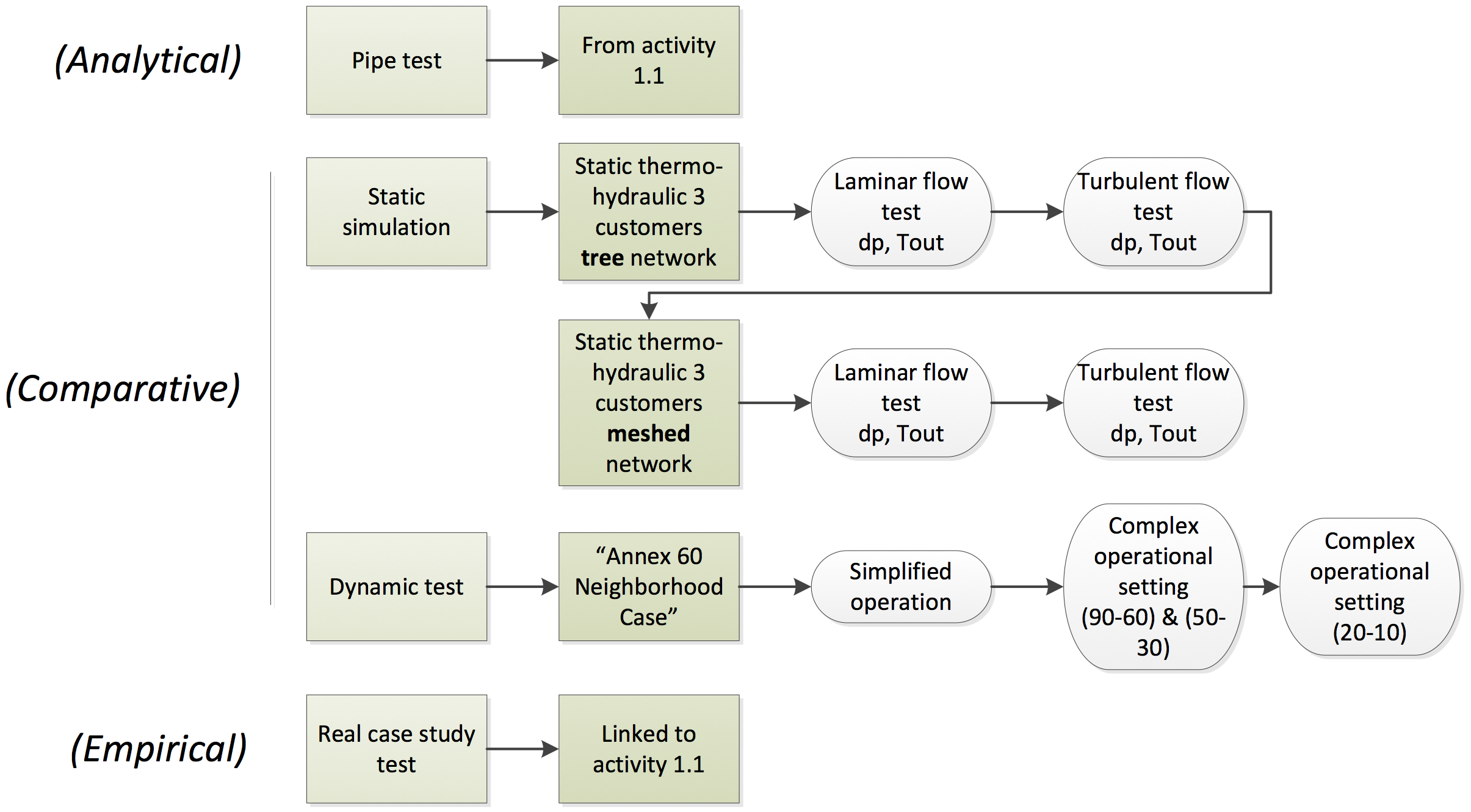
Fig. 10.7 Envisioned testing structure of the DESTEST Framework.

Focusing on heating and cooling distribution networks, the framework would build up from component tests such as a pipe. Starting with pressure drop validation for a pipe in steady state, levels of complexity can gradually be added, such as temperature drop, changes in mass flow, periods of zero mass flow and mass flow reversal, changes in inlet temperature and thermal capacity of pipe walls and insulation. In a next step, these components are added in a test grid set-up. At first, this is a purely branching network in a steady state (laminar or turbulent flow), thereafter meshed grids can be considered as well as dynamic operation. This case would correspond to the Annex 60 Neighborhood Case, which is described in the following section. Lastly, a database with measurements from a real district heating (and/or cooling) network could be built in order to simulate a realistic case and compare the outcome of the simulation with real measurements.

Finally, a range of key performance indicators has to be defined. These can be divided in different categories. First and foremost, the difference between the results from different models must be considered. Furthermore, the computational speed and memory needed for initialization and simulation are important. For the specific case of Modelica, other numerical parameters such as number of Jacobian evaluations, eigenvalues, number of states, size of non-linear systems etc. can be compared. It is important that for every test, a limited number of relevant key performance indicators is selected in order not to overcomplicate testing.

10.4.2. Definition of Common Exercise: Reference Annex 60 Neighborhood Case

10.4.2.1. Introduction

Activity 2.2 primarily focuses on evaluating, testing and demonstrating modeling and simulation approaches developed in Subtask 1. Therefore, the aim of this common exercise is to define a reference Annex 60 Neighborhood Case on which various of these models can be tested. The test case provides an environment enabling the analysis of aspects such as the following:

• Interconnection of electrical and thermal grids
• Hydraulic balancing
• Change from consumers to prosumers: influence of distributed energy generation
• Control strategies: their benefits, impact on consumers, modeling options
• Demand Side Management (DSM): how to use flexibility provided by thermal networks and storage

The development of the Annex 60 Neighborhood Case, comprises three steps described below. These steps aim at gradually incorporating features which are necessary to analyze the identified issues. During the course of Annex 60 not all steps were completed. Nevertheless this outline will serve as a guide for further development of the DESTEST.

In the first step, the description of the Annex 60 Neighborhood Case is elaborated. Considering the aims of this common exercise, a small neighborhood is defined, with typical configuration and providing possibilities to implement a district heating and electrical network. Buildings include residential dwellings and an office building, producing various demand profiles resulting from different use, size, insulation quality and occupancy. Description of a district heating network and an electricity network connecting all buildings is generated as well. The level of complexity of the simulated energy systems is progressively increased, from individual to collective complex systems.

The second step consists of modeling the behavior of buildings and their installations in the defined neighborhood, where buildings are treated as stand-alone (not coupled). Participants were asked to individually perform this task, freely selecting a building modeling approach, however, within the Modelica environment. Comparison of predefined performance indicators representative for the building energy demand is then carried out. While the main aim of this step is to identify a common library with building models, an additional aim is to demonstrate the consequences of modeling decisions and to illustrate the effect of different levels of complexity. By analyzing the results, the level of understanding in modeling buildings of all participants levels out, while corrections were performed to the developed models.

In the third step, district heating networks were investigated. Participants were asked to individually model the network, using models and simulation methods developed in other activities. For example, direct integration in Modelica may be chosen, or use of FMI and co-simulation. Reporting on the different approaches taken and modeling difficulties encountered, feedback is given to other activities, while knowledge is shared among participants.

10.4.2.2. Description of the Reference Annex 60 Neighborhood Case

This section provides an overview of the Annex 60 neighborhood case. A detailed description is available from the reference document at http://www.iea-annex60.org/downloads/Annex60_2_2_ReferenceCaseStudy-v1.0.pdf.

A typical neighborhood is defined including residential buildings and an office building. Mixing of end uses allows studying the potential heat exchange among buildings. Since the simultaneity of heating, cooling and electrical demand is a determining factor in the design and operation of district energy systems, additionally various insulation levels and stochastic user behavior are foreseen.

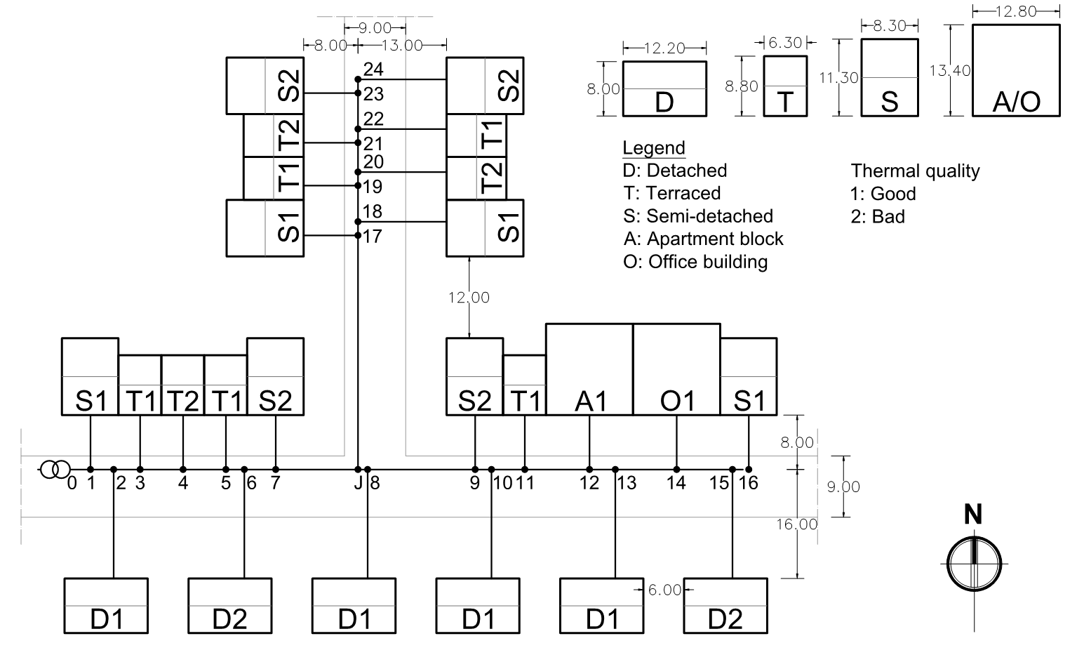
Fig. 10.8 Street layout of the neighborhood with the selected building typologies.

Neighborhood

The reference neighborhood is based on a small set of reference buildings which are combined to describe a street section. Five typologies are made for the building layouts, i.e. a detached (D), a semi-detached (S) and a terraced (T) dwelling, an apartment block (A) and an office building (O). Two sub-typologies are made to distinguish between the levels of thermal insulation. The five dwelling typologies and two levels of thermal insulation are combined into a street design of 24 buildings as shown in Fig. 10.8. All required piping and wiring of district systems (for heating, cooling or electricity) are foreseen on a single side of the street as shown in Fig. 10.8, resulting in asymmetric connections.

Building typology

Detailed plans of all five building typologies are given in the reference document describing all dimensions and interior subdivisions of the buildings. Such detail allows participants to select the number of simulated zones per building. Nonetheless, a minimum of two zones per building is required. Table 10.1 summarizes the main geometric parameters of the reference buildings. Each of the single-family residential building comprises two sub-topologies to distinguish between two levels of thermal insulation, the first one referring to the requirements of the EPBD 2010 in Flanders, and the second one representing typical Flemish buildings of the period 1946-1970, both based on the IEE TABULA project typologies. All construction elements are described in detail in the reference document, including material properties, angle-dependent glazing properties, and airtightness.

Table 10.1 Summary of the main building parameters (entire building for the dwellings and typical floor for the apartment block and office building, which have a total of 5 floors).

	Detached dwelling (D)	Semi-detached dwelling (S)	Terraced dwelling (T)	Apartment block (A)	Office building (O)
Usable floor area	102.7	100.9	107.5	107.5	107.5	\(m^2\)
Total floor area	185.5	187.8	161.0	161.0	161.0	\(m^2\)
Heat loss area	371.1	3051	219.1	104.6	104.6	\(m^2\)
Air volume	451.5	455.1	446.5	435.9	435.9	\(m^3\)

Occupancy

Initially, a constant set point temperature of \(21^{\circ}C\) for heating is assumed for all zones. There are no internal gains and no requirements for cooling. This simplification allows for an easier comparison between models and brings the focus on the implemented physics. In a next step, it is proposed to refine this assumption by introducing stochastic user profiles for internal gains, temperature set-points, electricity use, etc. All these are provided as input files for each building, based on generated profiles from the StROBe package of openIDEAS [BDCJ+15].

Space heating, hot water and ventilation systems

For the second step of this exercise, the energy demand is compared. Individual and ideal heating systems are assumed. State #1 residential buildings are heated by an air-to-water heat pump, while state #2 buildings are heated by a condensing gas boiler. There are no cooling systems installed in residential buildings. In the office building, the cooling load is covered by an air-cooled chiller and the heating load by a condensing gas boiler. The same simulation model of the condensing boiler is used for both residential and office buildings. Initially, the distribution and emission systems are not simulated. The condensing boiler, the heat pumps and the chiller are assumed to provide water at respectively \(50^{\circ}C\), \(40^{\circ}C\) and \(7^{\circ}C\). Nominal operation conditions for these systems are provided in the reference document, together with look-up tables for boiler efficiencies for the initial stages.

Reference district heating network

The district heating network topology considers the pipes for supply and return on a single side of the street, as shown in Fig. 10.8, buried at a depth of \(1 \, \mathrm m\). The pipes are buried directly in the ground. Three different scenarios have been considered, using different supply/return temperatures, namely:

• Scenario 90-60 has \(90^{\circ}C\) supply temperature and \(60^{\circ}C\) return temperature.
• Scenario 50-30 has \(50^{\circ}C\) supply temperature and \(30^{\circ}C\) return temperature.
• Scenario 20-10 has \(20^{\circ}C\) supply temperature and \(10^{\circ}C\) return temperature.

The pipeline distances between two nodes and the nominal diameter per scenario are specified, as are the insulation properties of the pipeline. The position of the main heat plant has to be considered at node 0. The temperature level of the different scenarios refers to the supply temperature at node 0 and the return temperatures at the costumers’ nodes. The DH design takes into account the maximum heat load requirements based on the space heating demand simulated in the previous steps, assuming a maximum velocity in the pipes of \(1.1 \, \mathrm{m/s}\).

The supply model can be initially considered as an ideal source supplying unlimited mass flow rate at \(90/50/20^{\circ}C\) respectively for the three scenarios. Therefore, an ideal pump is supposed to be installed, providing at any time step the required mass flow rate (no worst-point control on the pressure drop is considered).

Ground properties

The pipeline is assumed to be buried directly in the ground at \(1 \, \mathrm m\) depth. In order to calculate the ground temperature for the heat distribution losses of the pipe model, any ground model can be used. Ground properties and related assumptions are provided for uniform results among participants.

Substation design

Each substation contains a valve to control the water flow from the DH network and a heat exchanger between the primary loop (DH side) and the secondary loop (building side). The valve is controlled in order to meet the heat demand of the building and to maintain a low return temperature on the DH network side. The latter is the most important criterion in limiting the water flow and ambient heat losses in the DH network.

To model the heat exchanger, it is proposed to impose a constant heat transfer value (UA), to neglect the thermal inertia of the heat exchanger and to neglect the heat losses of the heat exchanger to the ambient. A set of equations to describe the substations is given in the reference document, resulting from the previous assumptions, as well as a proposed method to identify the parameters of each substation.

Demand

Participants not modeling the buildings in detail may use the provided heating demand profiles for the district heating simulation. The profiles were generated from detailed building simulations implemented at the KU Leuven, using this present description and the IDEAS Modelica library [BDCJ+15].

Model performance criteria

The developed models should be able to simulate a typical annual behavior of the buildings or district heating network. Depending on the models and simulators, not all performance criteria may be available. As a common base, we define the hourly data as the actual value at the beginning of the hour, and the hourly maximum (or minimum) as the maximum value of the above hourly data. The following model performance criteria should be evaluated.

Energy demand and energy use

The energy demand is the energy required by the building to achieve the set points regardless of the heating or cooling system. The energy use of the building takes into account the efficiency of the heating cooling system including conversion efficiency, control efficiency, emission efficiency and distribution efficiency. Initially, predefined system efficiencies are used for calculation of the energy use. The following information is required for model comparison, ideally at an hourly basis:

• Total and peak heating and cooling energy requirements of individual buildings and aggregated.
• Overall average system efficiency for each building.

Thermal behavior

The buildings are simulated in two ways: free floating temperature and with heating and cooling system. For both simulations, peak (maximum and minimum) and average temperatures are compared per dwelling. Ideally, hourly temperature profiles of each building for the free floating case will be available, to allow an additional analysis of the temperature rise and decrease.

District heating network

The following information should be provided:

• Minimum and maximum heat distribution losses
• Total energy for the heat distribution losses
• Minimum and maximum pressure drop
• Total ideal pumping energy

Production plant

The following information should be provided:

• Minimum, maximum and average mass flow rate
• Minimum, maximum and average return temperature
• Peak production
• Total energy production

LV distribution grid

Grid cable parameters

Three different grid strengths will be examined, denoted by strong feeder, moderate feeder and weak feeder. The nominal cross-section area of the cables is given in the reference document for all lines and each grid strength. For strong feeders 120 mm² cable is proposed for the entire grid; for the moderate 120 mm² for line 0-16 and 95 mm² for the branch J-24; and for the weak grid 95 mm² for 0-16 and 70 mm² for J-24 (see diagram Fig. 10.8). In practice, cables smaller than 70 mm² are rarely used.

The lengths of the cables between the LV distribution grid and buildings are shown in Fig. 10.8. The size of these cables is as follows:

• Single-family building (D/S/T): 16 mm²;
• Apartment building (A): 35 mm²;
• Office building (O): 50 mm².

The cable parameters are based upon the IDEAS library [BDCJ+15] and are given in the reference document.

Transformer parameters

Transformers are modeled with identical phase impedances for all three phases. The parameters are given in the reference document. For the strong and moderate feeders, a 250 kVA transformer is chosen, while for the weak feeder, a 160 kVA transformer is selected. This choice may vary depending on the load profile of the office building, and/or total grid load.

Single/three-phase connection

Buildings may have a single or three-phase connection to the LV distribution grid. Two options can be assessed:

• All buildings have a three-phase connection leading to balanced conditions.
• Buildings have a single or three-phase connection, depending on the power rating of loads in the building.

In the latter case, all buildings are single-phase connected to the LV distribution grid, except when the power rating of at least one load (e.g., heat pump or photovoltaic system) is larger than 5 kVA. This philosophy is taken from the connection requirements for PV systems in Flanders.

10.4.3. Annex 60 Neighborhood Case: a Comparative Study

10.4.3.1. Introduction

This section presents a comparison of the energy performance results obtained from the different approaches taken by activity 2.2 participants to model the common district case-study described in Section 10.4.2. The modelers (KUL, TUe, EDF, ULg) used the Modelica language and were given flexibility to choose their preferred modeling approach regarding model complexity, used libraries and components, etc. The aim of the exercise was to first predict the annual heating demand (peak and average) of the district, and then to analyze the differences in the results obtained by the different participants, evaluating the potential influence of their selected modeling approach.

10.4.3.2. Case Description

The Annex 60 Neighborhood Case was defined in Definition of Section 10.4.2. The main information is presented here for reader’s convenience. The neighborhood contains five typologies of building, i.e. detached (D), semi-detached (S), terraced dwelling (T), apartment (A) and office (O) building. Two levels of thermal insulation are taken into account. Level #1 represents the insulation level required by the EPB 2010 in Flanders and level #2 represents Flemish buildings in 1946-1970 based on the IEE TABULA report [CRHV11]. Fig. 10.8 depicts the street layout of the reference neighborhood. Detailed description about building layout, dimensions, thermal properties of building envelope please refer to case definition.

10.4.3.3. Modeling Approaches using Modelica

The models that constitute the district are based on different Modelica components libraries. The level of abstraction used to model the buildings and their sub-division in thermal zones as well as the heat transfer to adjacent buildings was left up to each of the participants. A constant heating set point of \(21^{\circ}C\) was used for all the buildings and no internal gains or shading were modeled. The assumptions and modeling approach adopted by the participants is summarized in Table 10.2.

Table 10.2 Summary of Modeling Approaches

Participant	TUe	EDF R&D	KUL	ULg	RWTH AACHEN
Libraries & Versions	Modelica 3.2.1 Buildings 1.6	Modelica 3.2.1; BuildSysPro 2015.12b	Modelica 3.2.1; IDEAS v0.2	Modelica 3.2.1; Buildings 1.5; Thermocycle	Modelica 3.2.1; AixLib v0.3.2
Nb. of Zones	1 per floor (D, T, S); 2 per floor (O); 3 per floor (A)	Monozone	1 / floor (unheated attic ) (D, T, S); 3 per floor (A,O)	6 (D, T); 5 (S); 5 per floor (A,O)	4 (D, T, S, A, O)
Shading	N	N	N	N	N
Heat transfer through adjacent surface
Floor to Ground	Y	Y	Y	Y	Y
to adjacent zones	Y	Y	Y	Y	N
to adjacent building	Y	Y	N	N	N
Ground Floor Temperature (oC)	10.3	10	9+periodic effect (ISO 13370)	10.0	10
Weather Location	Uccle, Belgium

10.4.3.4. Results and Discussions

Figures 10.9 to 10.15 show the heating demand simulated by the participants for the different building typologies in the reference neighborhood. To better present heating demand for each building typology, we divided the results into a cold and warm season according to the outdoor air temperature from the weather file and the heating set point used. The warm season was defined from the first day when the outdoor air temperature was greater than the heating set point to the first day when every hour was lower than the set point. In this case, this period goes from the 19th of May to the 10th of October. The cold season was assumed to be the remaining time of the year.

Figures 10.9 to 10.15 present a comparison of the thermal performance of the different building typologies for the cold season. The apartment block (Fig. 10.9) and office building (Fig. 10.10) appear to have similar performance. The differences are only \(1.4\%\) on average demand and \(0.1\%\) on maximum demand for the results from TUe. This is mainly due to the similar geometry and thermal properties used for both building envelops. Note that internal gains were not included in the model. The different modeling approaches by the participants in terms of the number of thermal zones modeled and the heat flow between adjacent buildings (Table 10.2) did not create significant differences. However, for other building typologies, significant differences can be observed, especially for the poorly insulated buildings.

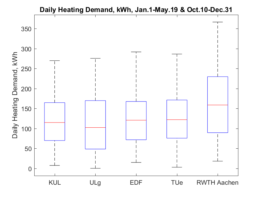
Fig. 10.9 Simulated daily heating demand apartments

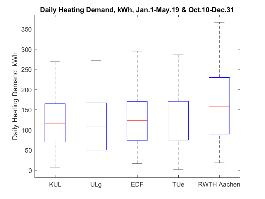
Fig. 10.10 Simulated daily heating demand for offices

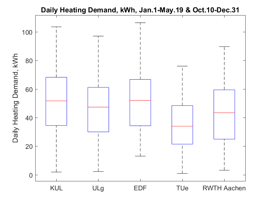
Fig. 10.11 Simulated daily heating demand for detached dwellings

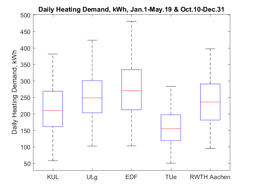
Fig. 10.12 Simulated daily heating demand for semi-detached dwellings S1_1

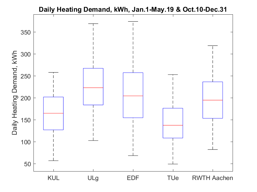
Fig. 10.13 Simulated daily heating demand for semi-detached dwellings S2_7

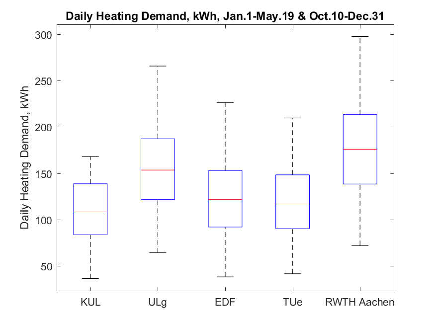
Fig. 10.14 Simulated daily heating demand for terraced dwellings T1_3

Fig. 10.15 Simulated daily heating demand for terraced dwellings T2_4

One of the reasons for these differences could be the approaches taken to model the heating system. Fig. 10.16 shows indoor air temperature in the semi- detached dwelling S1_1 from ULg and TUe. The results from ULg show room temperatures varying from \(20.4\) to \(21^{\circ}C\), with an average of \(20.6^{\circ}C\). From the TUe results, we can observe that room temperature was most of the time at \(21^{\circ}C\), due to the idealized heating control modeled.

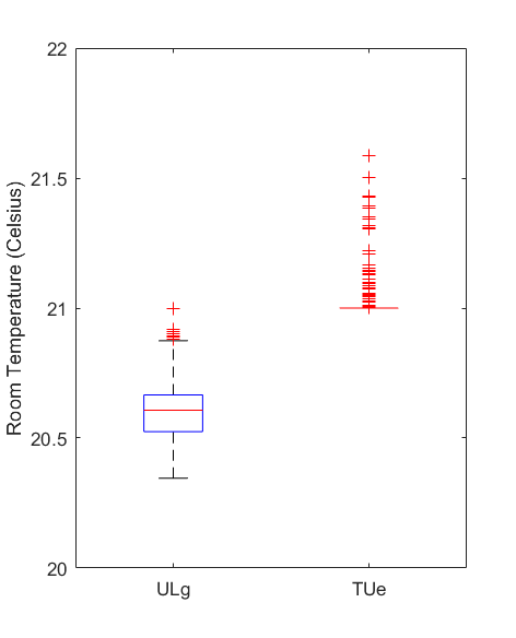
Fig. 10.16 Simulated room temperature for semi-detached dwelling S1_1

Figures 10.17 and 10.18 show annual heating demand and peak demand per building of the district. Significant differences can be observed in poorly insulated buildings such as buildings 4, 6, 7, 9, 15, 20, 21, 23 and 24. These results are much more sensitive to the complexity and assumptions adopted in the modeling approach. We can also observe different results for two buildings of the same typology, as for numbers 17 and 18. The difference in heating demand is caused by the way the heat transfer to adjacent buildings is modeled.

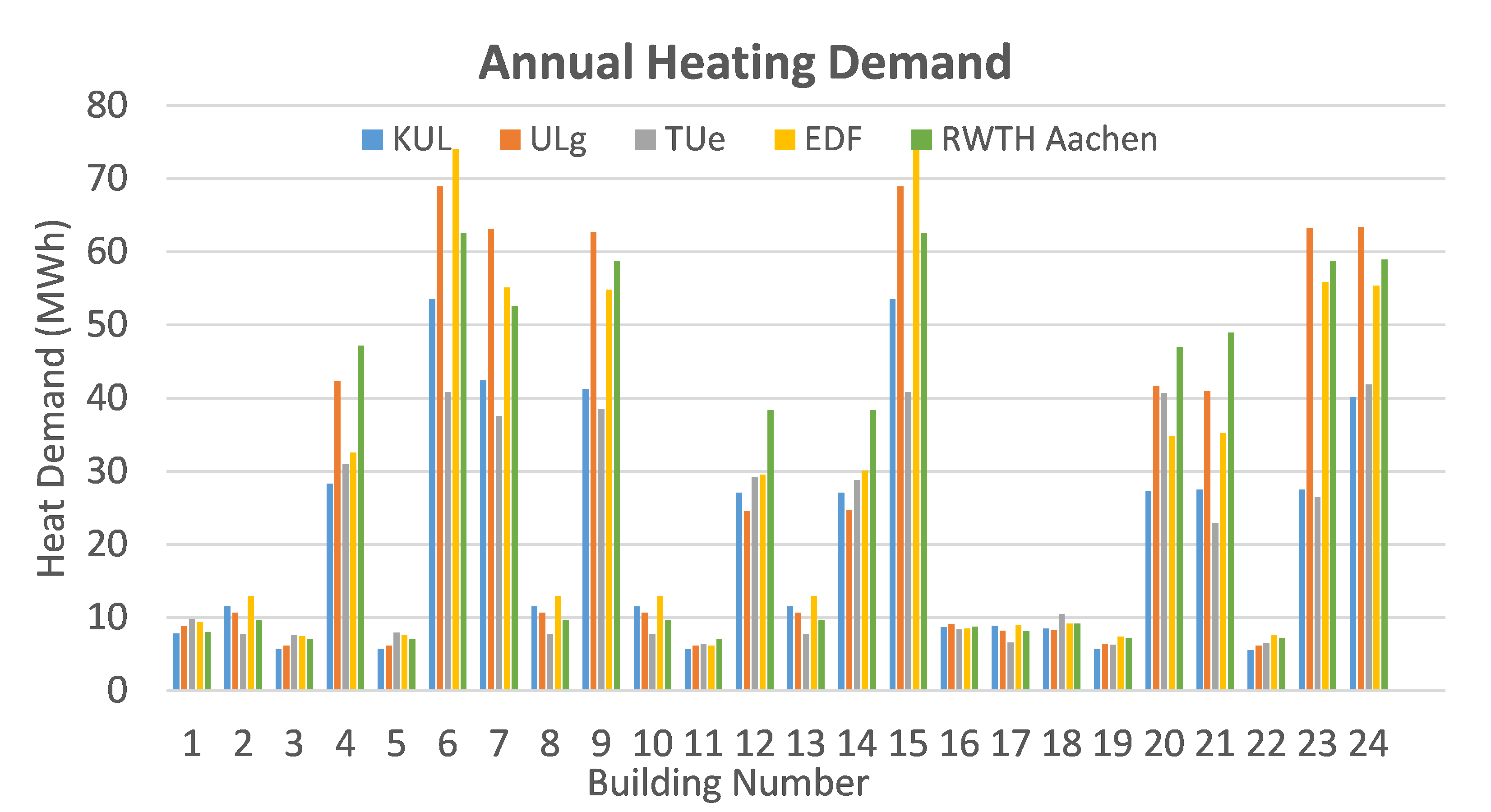
Fig. 10.17 Simulated annual heating demand for each building from the different participants

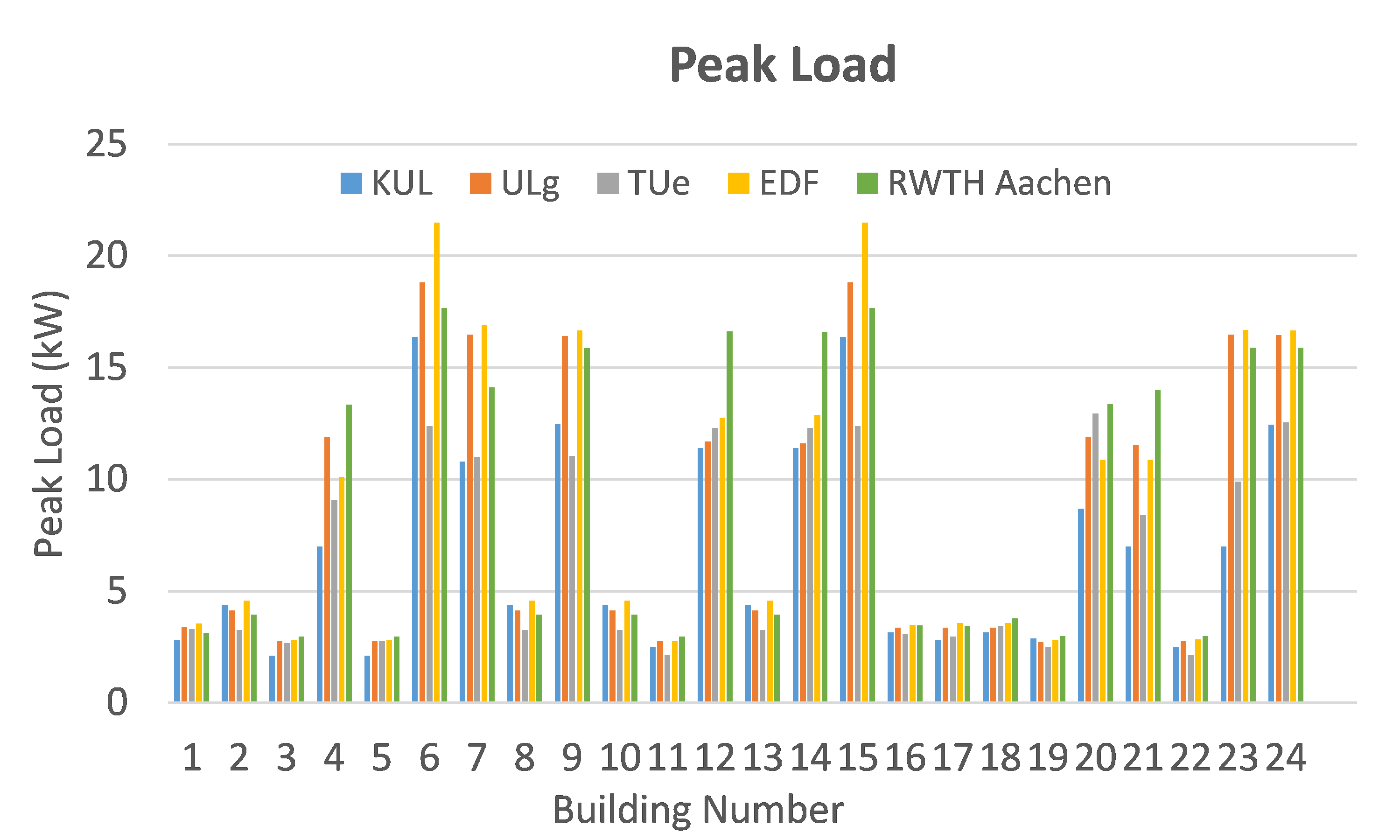
Fig. 10.18 Simulated annual heating peak load for each building from the different participants

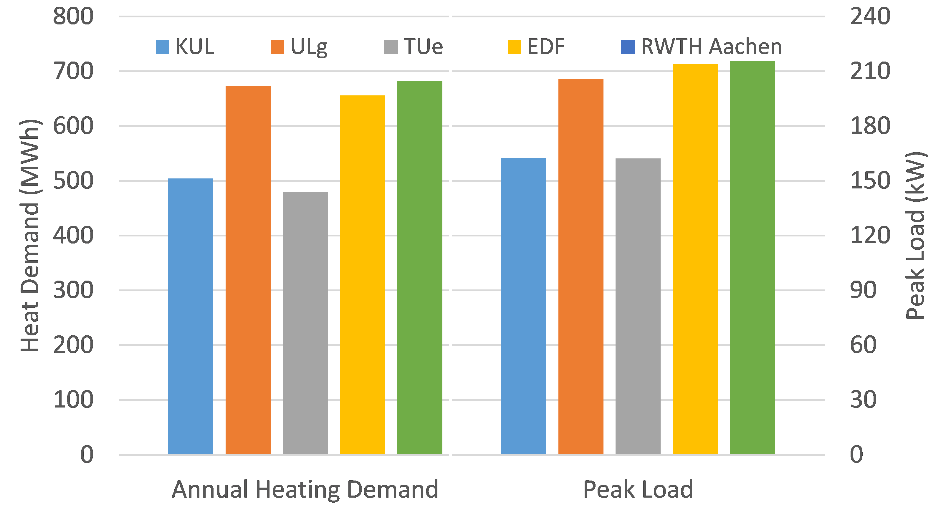
Fig. 10.19 Overall yearly annual heating demand and peak load on the Annex 60 Neighborhood Case

Figure 10.19 shows the overall heating demand and peak load from the different participants. As for the building analysis on figures 10.17 and 10.18, we can see that KUL and TUe may have underestimated energy needs with respect to other participants. The results show significant deviations for the overall yearly heating demand up to 20% from the average and 15% for the peak heating demand.

In order to further compare the simulated results from different participants, energy signatures for one building representative of each building typology are generated and shown in Figures 10.21 to 10.24. The energy signature shows the relationship between the outside air temperature and heating demand for a given building. A linear regression of daily average values was performed for every building typology.

Taking the energy signature of the detached dwelling (Fig. 10.20) as an example, the relationship between daily heating demand and daily average outdoor temperature can be observed. This relationship consists of two parts, one where it is approximately constant (flat) for all temperatures above the balance temperature (when the set-point is reached without the need for heating) and a part with certain slope for outdoor temperatures when heating is required. A linear regression for these temperatures above the balance temperature is shown in Fig. 10.21. R-squared for the three regression curves range from \(0.72\) to \(0.78\).

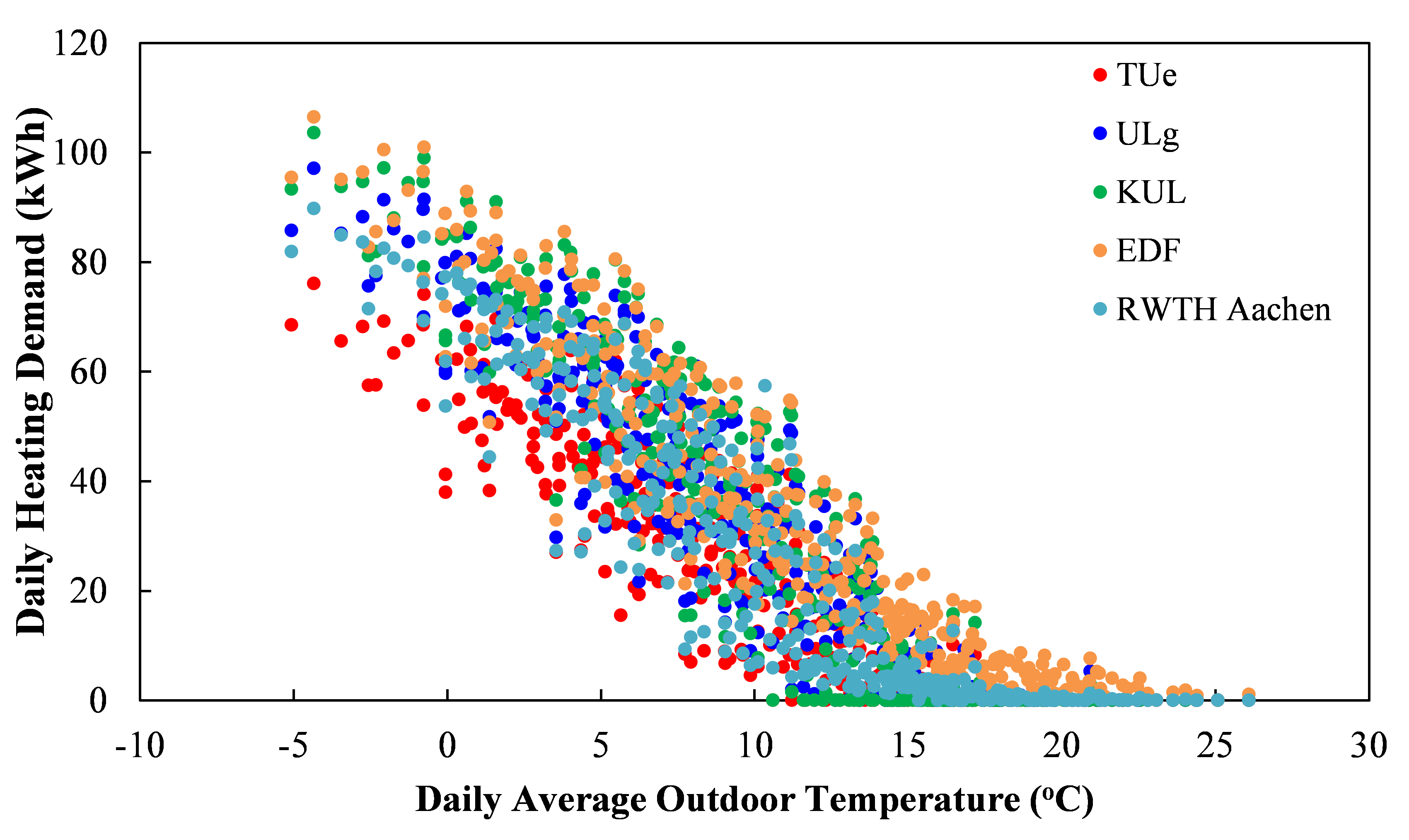
Fig. 10.20 Relationship of simulated daily heating demand for D1 and outdoor temperature by different participants

The energy signatures for all other building types of thermal insulation level 1# are shown in figures 10.22 to 10.24. As depicted from figures 10.9 and 10.10, heating demands in the apartments building (A) and office building (O) have similar distributions. As stated before, this is mainly due to not including internal gains and a similar set point schedule. For this reason, only the energy signature of the apartments building is shown (Fig. 10.22). Only one building per typology is illustrated, in this case, terraced house no.11 and semi-detached house no.1. The terraced dwellings have the largest observed difference between participants. Both slopes and balanced temperatures vary significantly. This could be explained by the way heat transferred is modeled across adjacent buildings, since terraced house no.11 has a larger heat transfer surface to adjacent buildings compared to its own volume.

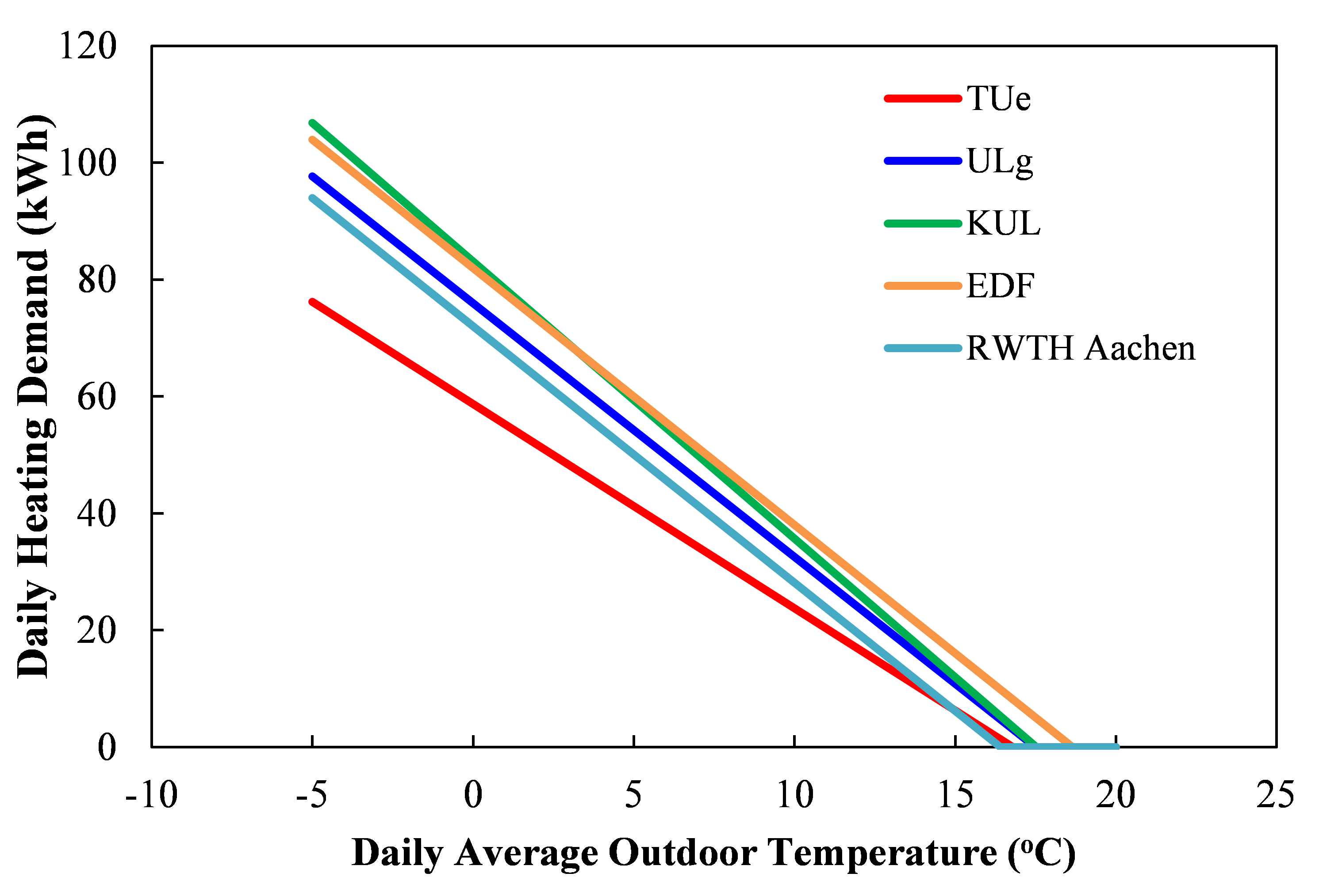
Fig. 10.21 Energy signature for building type D1

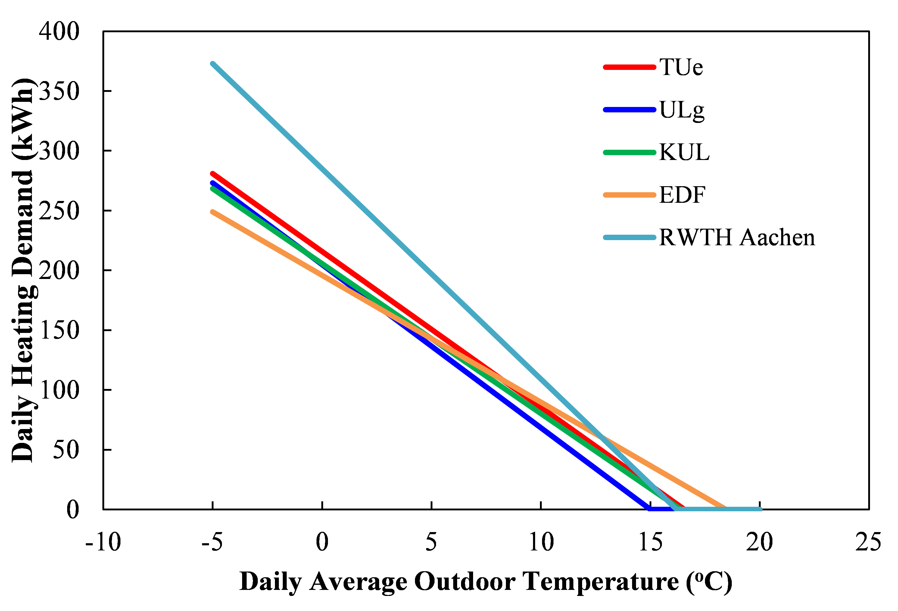
Fig. 10.22 Energy signature for building type A

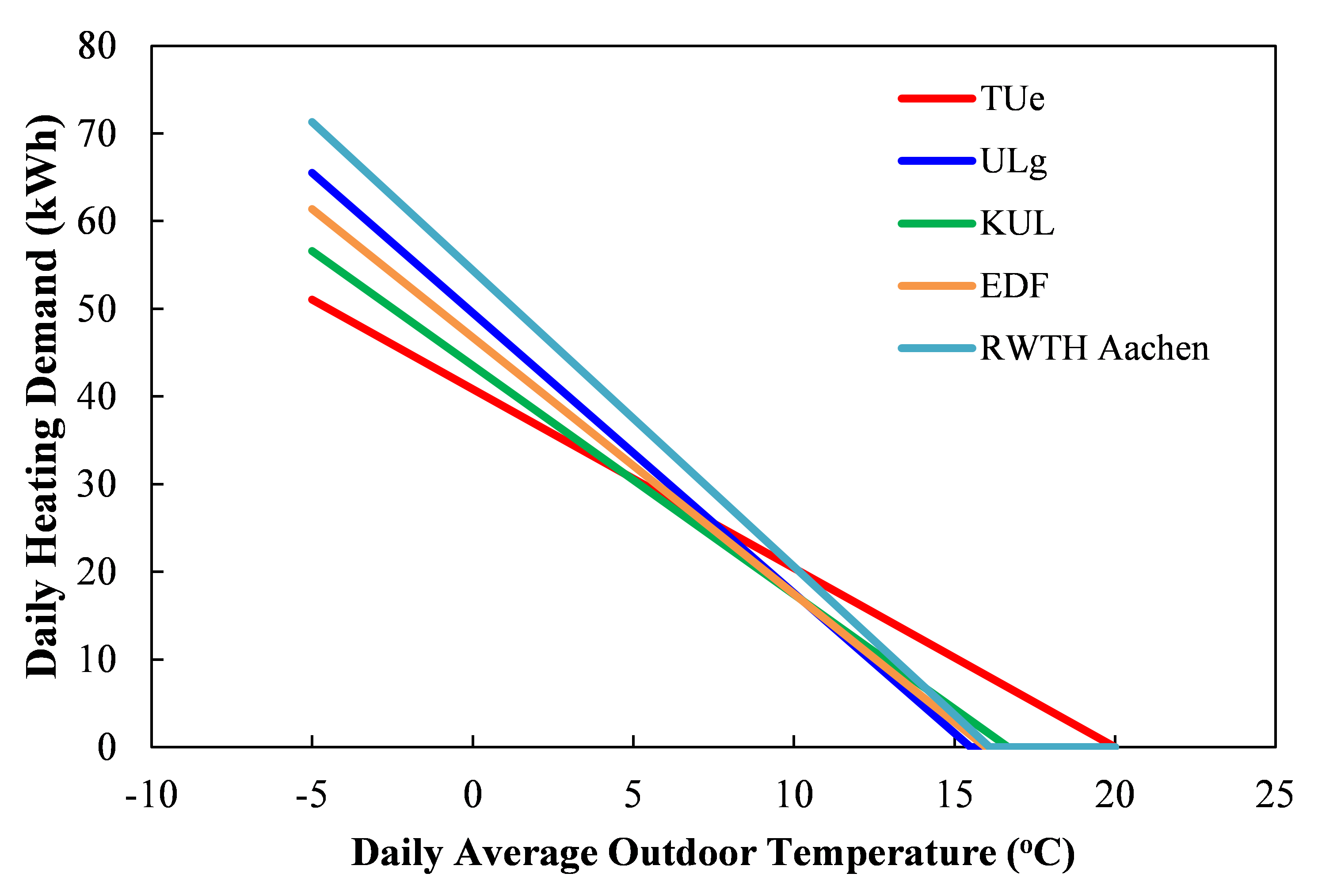
Fig. 10.23 Energy signature for building type T1

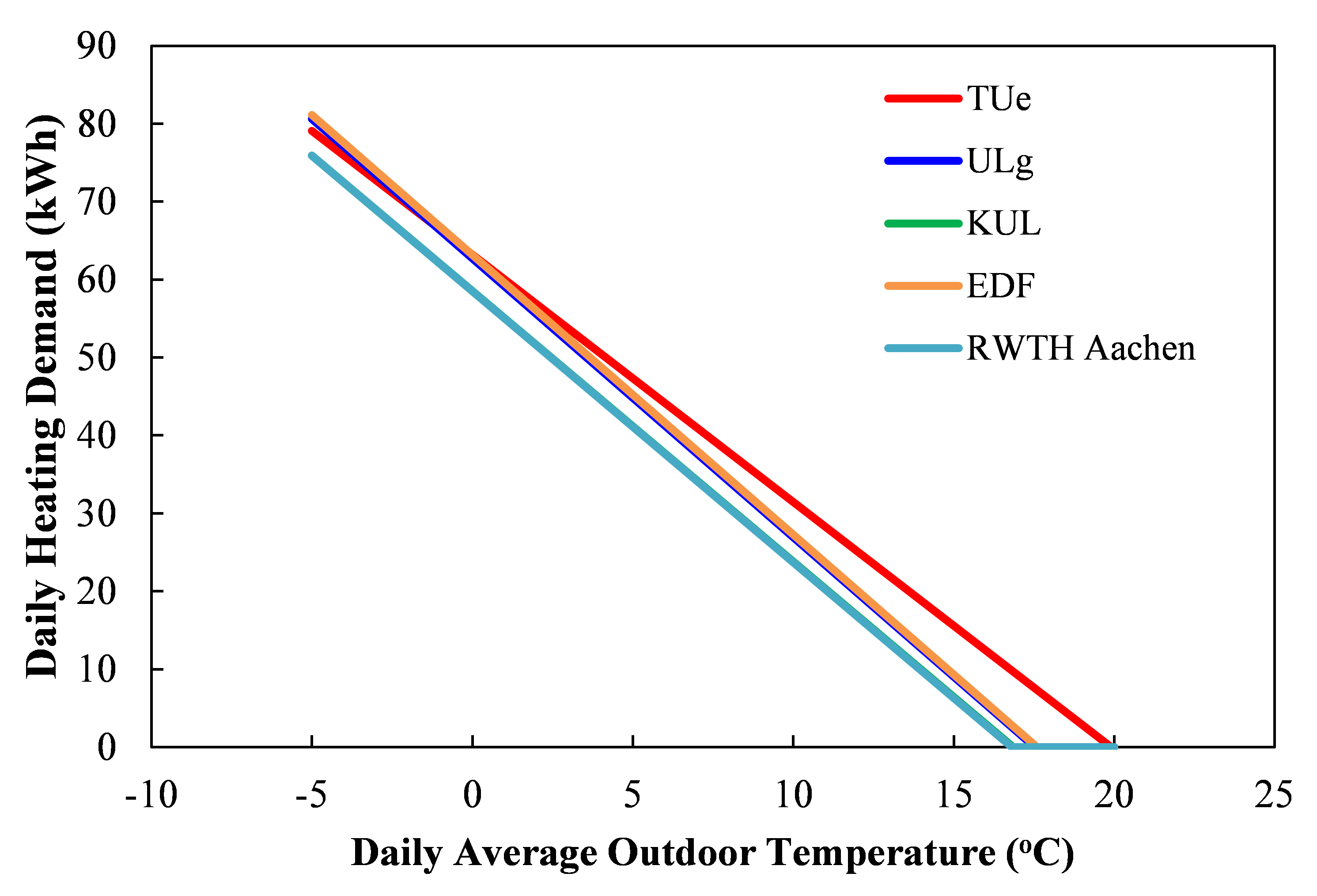
Fig. 10.24 Energy signature for building type S1

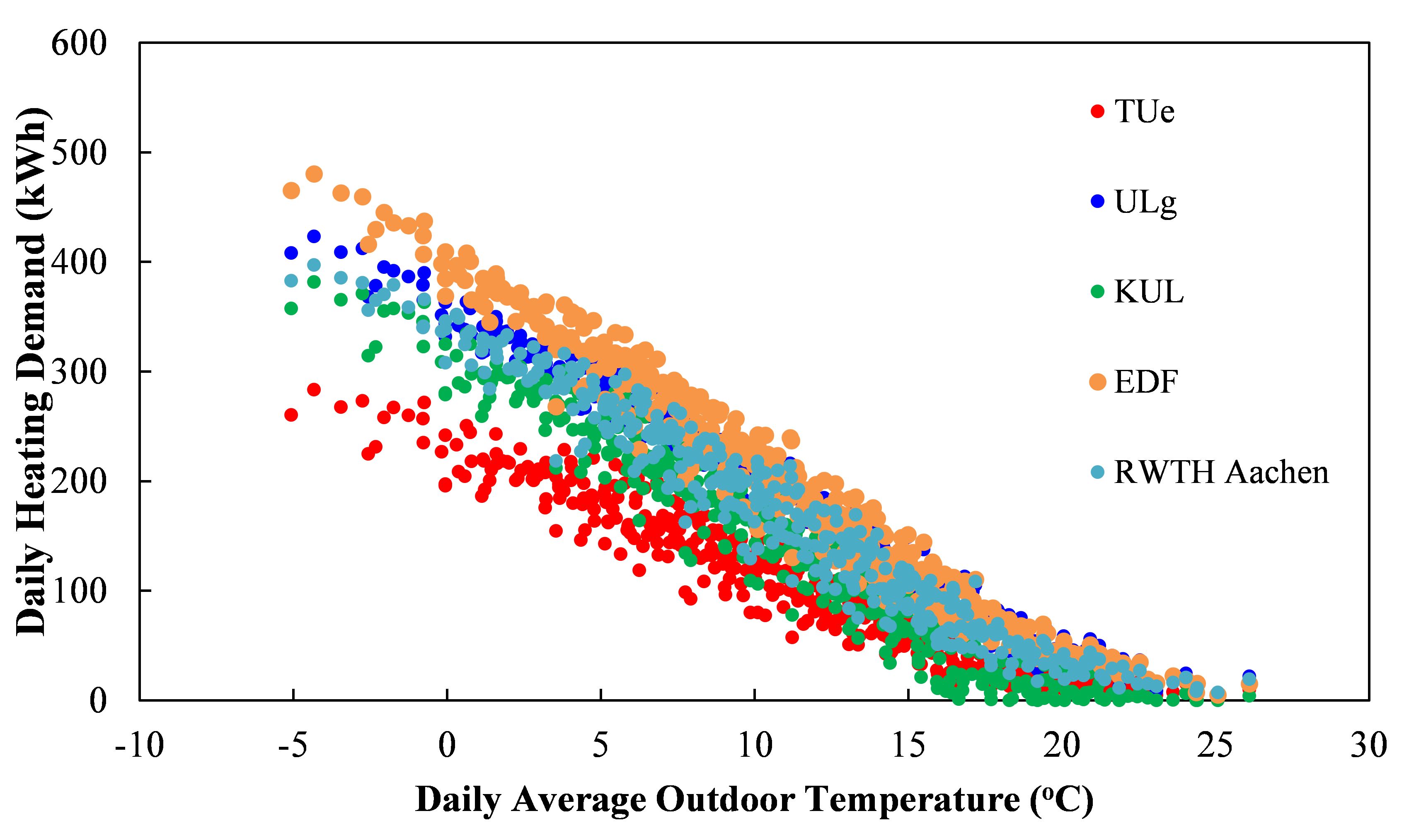
Fig. 10.25 Relationship of simulated daily heating demand for D2 and outdoor temperature by different participants

In addition, Figures 10.25 to 10.28 show the energy signature generated from the simulated data obtained by the participants for buildings with thermal insulation level #2. Compared to Fig. 10.20, the linear relationship between daily heating demand and daily average outdoor temperature is more obvious and, as expected, the balance temperature of poorly insulated buildings is significantly higher, as shown in Fig. 10.25. The energy signature of each building typology with thermal insulation level #2 are shown in figures 10.26 to 10.28.

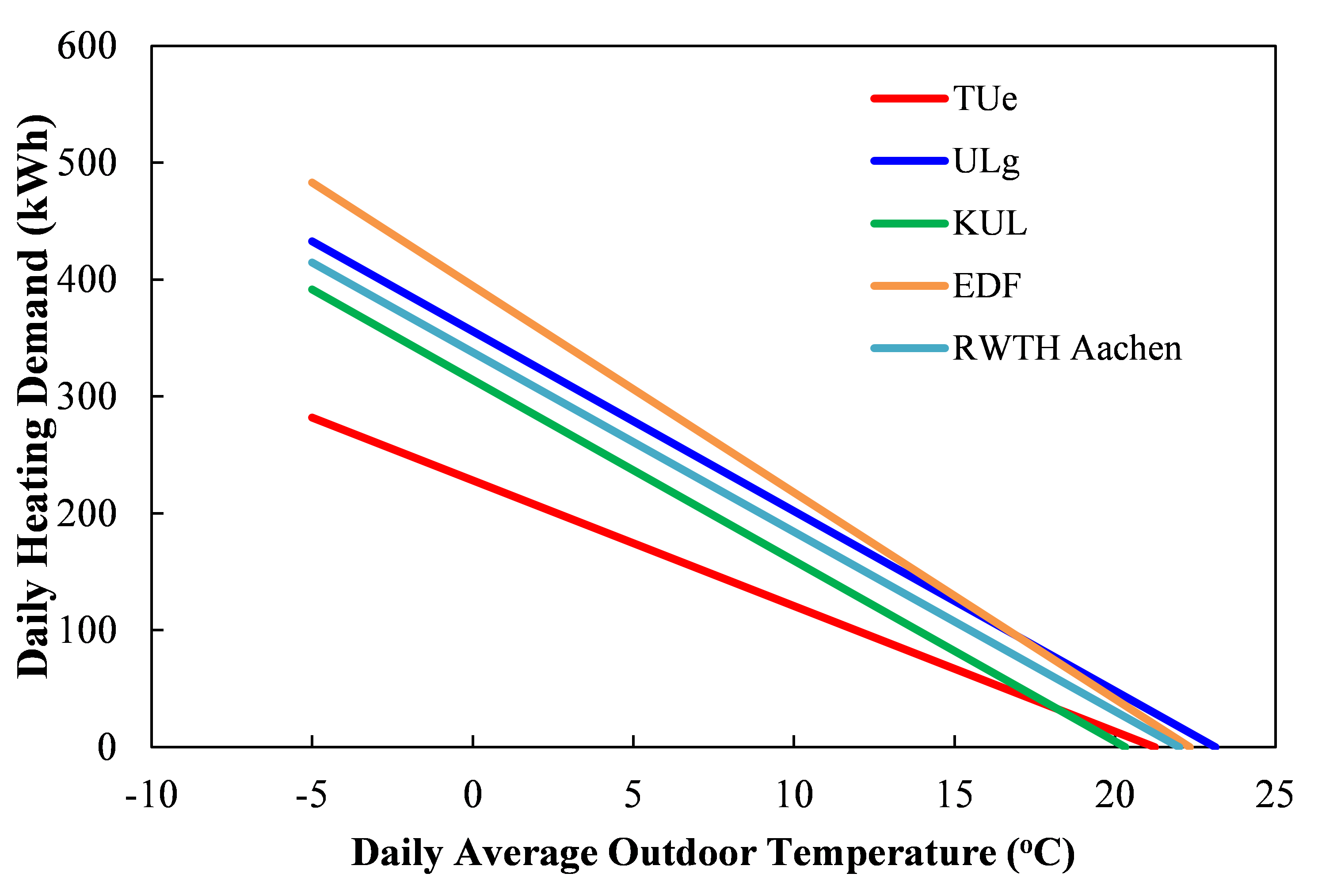
Fig. 10.26 Energy signature for building type D2

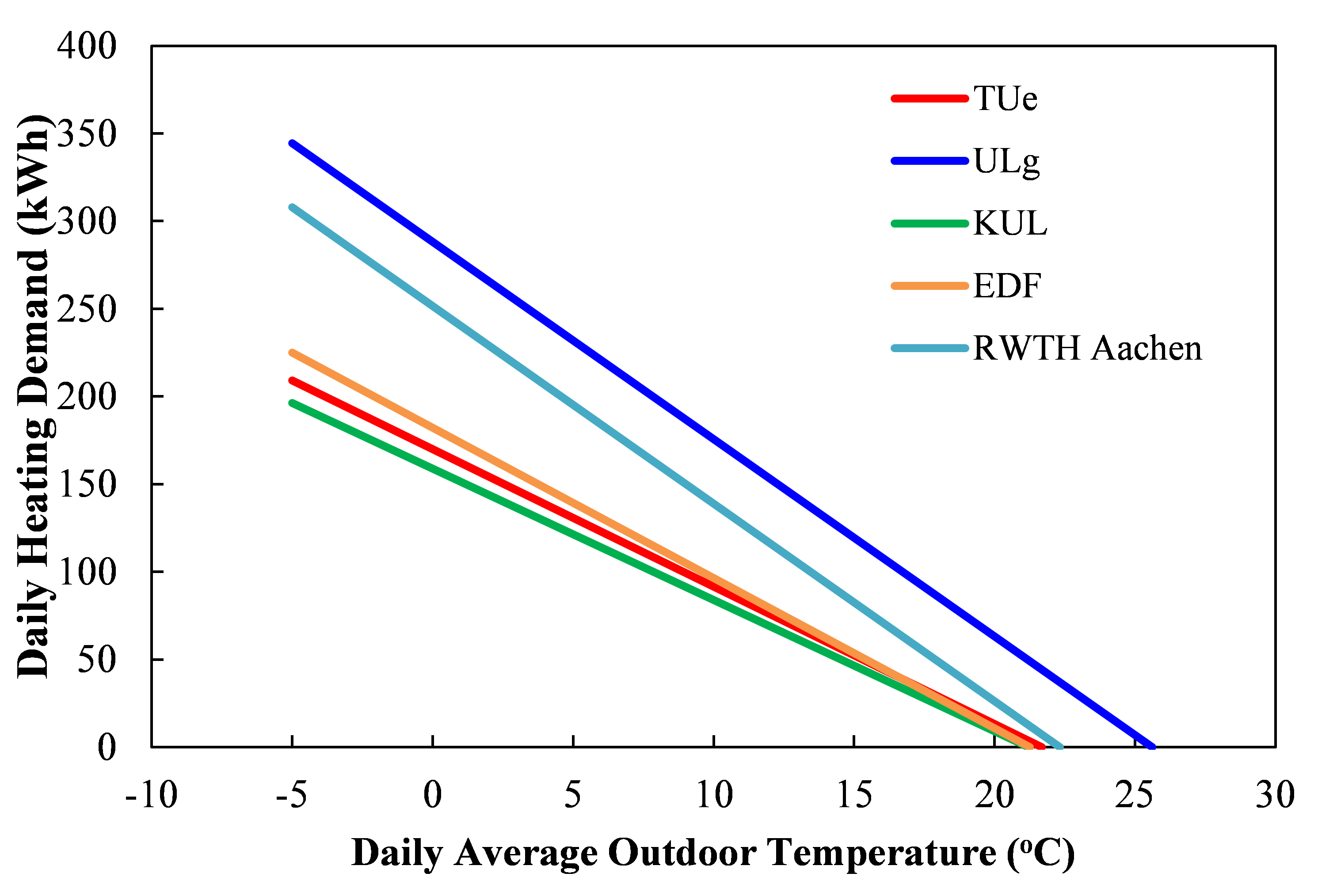
Fig. 10.27 Energy signature for building type T2

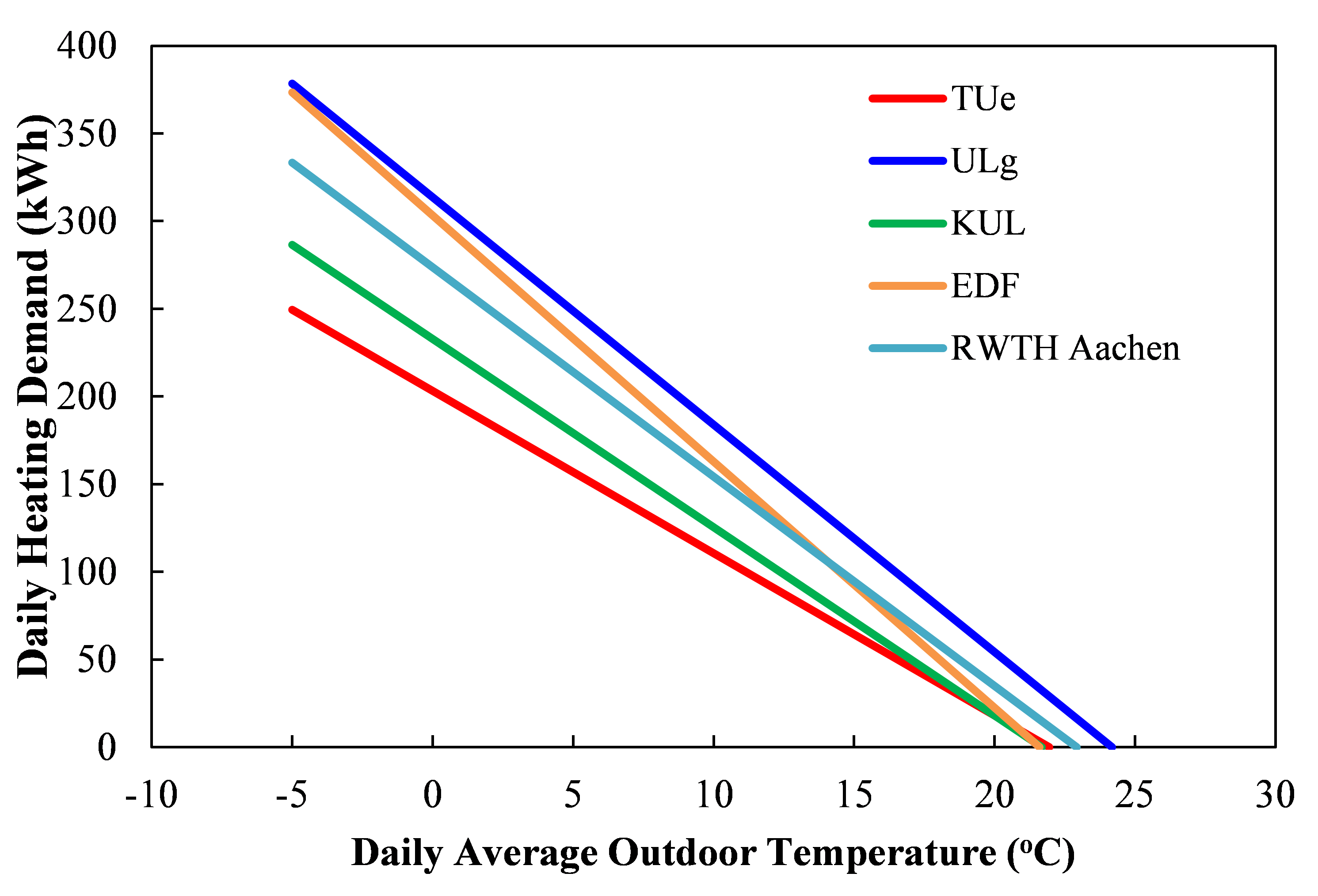
Fig. 10.28 Energy signature for building type S2

10.4.3.5. Summary and Discussion of the Common Results

Five participants from different institutions modeled and simulated the Annex 60 Neighborhood Case using different approaches and Modelica libraries. As illustrated and discussed in previous sections, the largest relative differences on heating demand among the participants occurred in poor insulated buildings. A preliminary analysis has been conducted to explore the possible causes, which can be concluded as follows:

• Relative to the selected modeling approaches, e.g. zoning methods, heat storage for internal partitions, heat transfer through surfaces (from adjacent zones and buildings), soil temperature, thermal models;
• Relative to the parameters selected, e.g., geometrical dimensions were provided as detailed floor plan with thickness of walls. However, modelers may have used different measuring approaches regarding outside/inside/center of the walls;
• Undefined inputs, e.g. infiltration rate for non-conditioned zones, thickness of glass pane and air space.

However, within this project, we could not conclusively determine where the discrepancies origin from. Therefore, one suggestion for further research is to conduct a systematic evaluation, e.g., a one-at-a-time analysis. It would be interesting to additionally perform a sensitivity analysis with respect to the mentioned parameters. Further evolution of the DESTEST to compare the energy performance results obtained from different modeling approaches will require that the case descriptions avoid ambiguous specification of parameters.

10.4.4. Examples of the Use of the Annex 60 Neighborhood Case

In this section, we briefly present two examples of the use of Annex 60 Neighborhood Case that extends the above performance studies. They were directed toward bioclimatic design and retrofit solutions for DHS extension respectively. The following results are mainly preliminary and will be further described and analyzed in future work.

10.4.4.1. Towards Urban and Bioclimatic Design: Taking the Building Surroundings into Account

The ANR VALERIE collaborative project (2009-2012) adopted a bioclimatic approach of building analysis to understand the possible energy exchanges (like infra-red radiation) of the building with its neighbors, shading effects or urban heat island effects [Duf12]. Results showed that current design methods under-use these available resources. Thus, the source of performance brought by the use of free renewable energy available in the environment is more significant than “more insulation” for new buildings [CDRR12]. Urban densification is also a major factor of urban micro climate degradation, and specialists of urban issues seek more information on the influence of buildings. In order to study these new research questions, the ANR MERUBBI project (2014-2018) is developing a methodology that takes the urban aspect into consideration by dealing with the integration of a new building into an existing district.

The new tool chain developed in order to answer these research questions has been applied to the Annex 60 Neighborhood Case. Starting from the common neighborhood description, the district was modeled using SketchUp. Then, the 3D architectural model is transformed into an energy model in two steps. The first one consists of a transformation of the 3D architecture model into a pivot XML file. Then, a Python tool has been developed to translate the gbXML file into a building energy model based on the BuildSysPro open-source Modelica library [PKL14]. Raytracing calculations, based on the open-source Embree library [WWB+14], are used to calculate the form factors in the district, and the amount of direct, diffuse and reflected solar radiation for each surface, as well as the ground albedo.

At the time of this writing, only preliminary results could be established and analyzed. These show that, for instance, that certain houses are negatively impacted by the presence of nearby apartment blocks, showing an increase of 20% of their heating energy consumption. This preliminary work will be detailed further when the tool chain of the ANR MERUBBI project is fully validated.

The impact of shadow effects is small for the configuration of the Annex 60 Neighborhood Case. Hence, it is not necessarily the best test case to assess the effect of local micro climate effects. Nevertheless, it was found useful to perform preliminary tests. It however demonstrates that in order to develop a meaningful DESTEST, different use cases should be carefully analyzed to make sure that the developed DESTEST is suitable to assess the analyzed problem. This example showed that it the development of more than one neighborhood case description may be necessary to cover the variety of problems that may be encountered and assessed in district energy simulations.

10.4.4.2. Model-Based Assessment of Cost-Effective Retrofit Solutions for a District Heating System Extension

Numerous research has been conducted on DHS, early examples go as far as the 14th century. However, few studies can be found on the evolution and the adaptation of older DHS in today’s world. Therefore, the present study adopted the Annex 60 Neighborhood Case to define a fictional neighborhood for the investigation of the long-term adaptability of such an existing DHS. In particular, we considered reusing the return water of the existing network to heat a new branch of the DHS, as shown in Fig. 10.29.

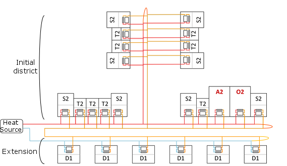
Fig. 10.29 Diagram of the studied district based on the Annex 60 Neighborhood Case. Red lines represent the supply flow, orange lines the intermediate flow, and blue lines the return flow. Buildings A2 and O2, in red, are assumed to belong to the municipality. The curves connecting supply and return lines represent the bypass valves.

The upper part indicates the initial DHS (red and orange pipes), which is directly fed by the heat source. The lower part shows the extension branch to be added to the initial DHS (orange and blue pipes), which will be fed by the return water of the initial DHS. In this study, some promising retrofit opportunities were evaluated on an extended DHS. In particular, the following stand-alone retrofit measures were applied in the original study :

0. No retrofit measure.
1. Retrofit of the envelope of the municipality buildings.
2. Decentralized storage in each of the new buildings.
3. Centralized storage on the municipality buildings.
4. Limitation of the internal set point temperature.

Studies were done to compare the results to the new DHS without any retrofit measures (solution #0) during the coldest week. Solution #1 allows significant energy savings, and thus presents better results to extend the network up to a certain point. Installing individual and centralized water tanks (retrofits #2 and #3) present a global increase of the energy demand of the DHS. Preliminary results show that, during the peak demand, the DHS is unable to supply enough heat to the customers, regardless of the retrofit measure. As a consequence, during the peak laod, we observe a maximum deviation of \(1.12\) Kelvin with respect to the set point temperature.

This study is an example of how the Annex 60 Neighborhood Case has been used as a case to analyze possibilities for retrofitting of an existing DHS.

10.5. Multi-Physics Simulation of DES in Modelica

This example demonstrates how Modelica allows to couple models of different physical domains for voltage stabilization of the distribution grid through demand response and PV inverter control. The example analyzes both the thermal and electrical dynamics of a small neighborhood with a high PV penetration. It requires the coupling of models for building energy simulation, electrical system simulation and feedback control loops. The models interact with each other through the electrical load imposed by the building on the grid, and the feedback control that adjusts the building room temperature set point and that increases the reactive power of the PV inverter in case of violation of the power quality.

Fig. 10.30 Neighborhood model with renewable energy sources. The yellow lines are weather data, green lines are electrical lines, and dashed blue lines are for post-processing.

Fig. 10.30 shows a net zero energy (NZE) neighborhood. By coupling models of buildings, HVAC, electrical systems and controls we can assess the effect of building load onto the electrical grid and assess the efficacy of control measures. The neighborhood contains seven small office buildings. Each building represents a small office that is part of the EnergyPlus commercial reference building models [DFS+11]. Each model has one floor and is divided into five thermal zones plus one attic. The floor area of each building is about \(500 \, \mathrm{m}^2\).

The building model comprises four different components, the thermal part, the schedules, the HVAC system and the electrical models. The thermal part accounts for the heat transfer through the envelope and energy storage in building constructions. The schedules represent the building internal loads due to occupants, as well as plug loads and lighting systems. The HVAC model represents the mechanical system and the control loops that maintain the thermal comfort in the building. The electrical models represent the interaction between the building and the electric network. They include an inductive load model that represents the electric load of the building and PV panels. All models are implemented in Modelica using the Buildings library [WZNP14][BWN14]. The thermal model was available as an EnergyPlus model. To integrate it with the rest of the building model, it was automatically converted to Modelica. The automatic conversion program leverages the OpenStudio API to identify the thermal zones and the components of the building fabrics. The conversion program converts the models by instantiating and connecting components of the Modelica Buildings library.

The building electricity consumption is modeled using the inductive load

\[\begin{split}P_{bui}(t) &= P_{hvac}(t) + P_{plug}(t) + P_{light}(t), \\ Q_{bui}(t) &= P_{bui}(t) \tan(\phi),\end{split}\]

where \(P_{bui}(\cdot)\) is the total active power, \(Q_{bui}(\cdot)\) is the total reactive power, \(\phi\) is the phase angle of the apparent power for the power factor \(p_f\), with \(\phi = \arccos(p_f)\), \(P_{hvac}(\cdot)\) is the power consumed by the HVAC system, \(P_{plug}(\cdot)\) are the plug loads and \(P_{light}(\cdot)\) is the lighting power. In addition, the neighborhood has a wind turbine that supplements the energy provided by the PVs. TMY3 weather data for San Francisco, CA, were used. For more information about the electrical models and their implementations see [BWN14].

The nominal voltage of the neighborhood is \(V_{nom} = 1.2 \, \mathrm{kV}\) and the nominal load of each building is \(P_{nom}^{load} = 18.6 \, \mathrm{kW}\). The total nominal power of the PVs installed in the neighborhood is \(P_{nom}^{PV} = 130 \, \mathrm{kW}\) and hence twice the sum of the nominal load of the office units. The PVs are unevenly distributed among the different buildings. The nominal power of the wind turbine is \(P_{nom}^{wind} = 93 \, \mathrm{kW}\) and therefore it is five times the nominal load of an office building. The buildings are connected through annealed aluminum cables of size AWG 1/0 that are \(300 \, \mathrm{m}\) long. The neighborhood produces annually about \(25\%\) more energy than it consumes.

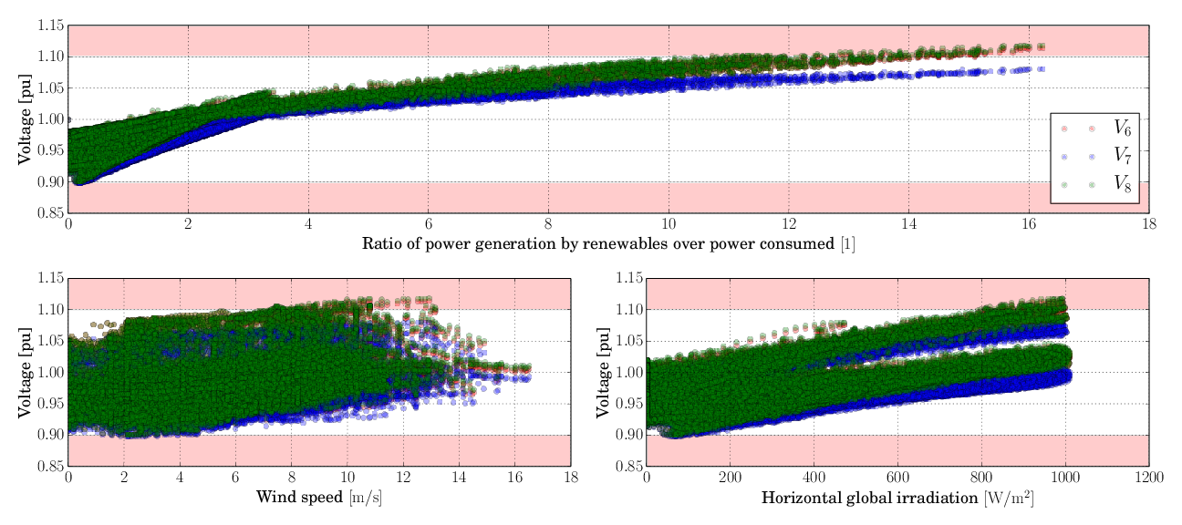
Fig. 10.31 Voltage levels in three different nodes of the neighborhood as a function of power generated by renewables, wind speed and horizontal global irradiation without feedback control.

We assumed the electrical system to be balanced because the analysis does not focus on possible asymmetries caused by the connection of the loads and sources on different phases, but rather on their impact on the voltage quality. In particular, we aim to keep the voltage within an admissible region of \(V = [0.9, \, 1.1]\) pu. To obtain diversity, the PV efficiency, orientation and tilt angles have been varied. Also, the power factor of the inductive load varies among the buildings between \(0.8\) and \(0.95\).

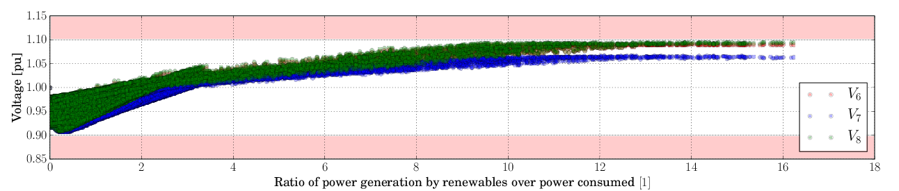
Fig. 10.32 Voltage levels in three different nodes of the neighborhood as a function of power generated by renewables with feedback control that adjust room air temperature setback and reactive power control at all PV inverters.

We will now analyze the simulation results for the case where there is no control to ensure that the voltage remains within the admissible region. Fig. 10.31 shows how the voltages in three different nodes of the neighborhood vary with respect to the power generated by the renewables over the power consumed. The lower two plots show the voltage at the three nodes as a function of wind speed and horizontal global irradiation. As expected, the voltage increases as the power generated by the renewables increases. The highest voltage is \(V_8\), measured by the sensor sen8 in Fig. 10.30, which is at the end of the line where the concentration of PVs is higher and where the wind turbine is located. During \(17\) hours of the year, the voltage is above or below the admissible region of \(V = [0.9, \, 1.1]\) pu.

Fig. 10.33 Electrical circuit with reactive power control at the PV inverter.

To keep voltages within the admissible region, we will now add two control measures to the above example. During low voltages, we increase the set point temperature of the buildings by \(2\) Kelvin. During high voltages, we add reactive power at the PV converters [TSBC11]. Fig. 10.33 shows the section of the Modelica model that comprises of the building load, the PV, and a reactive load. Based on the voltage at the PV connection, a feedback controller injects reactive load in order to not exceed a voltage set point of \(1.09\) pu. Fig. 10.32 shows that this control measure keeps the voltage within the admissible region.

10.6. Co-Simulation of DES

Co-simulation defines a technique that allows simulators to be executed simultaneously while exchanging data during run-time. It allows a coherent integration of a decomposed system by assigning a specific solver to each sub-component. Thus, co-simulation methods can provide a solution to address performance limitations that may be encountered when simulating the overall system in one tool. Furthermore, co-simulation allows reuse of domain-specific tools.

In this section, we propose a practical application of co-simulation and tools described in Section 6, by applying it to a simple DES test case using a limited number of dwellings. The model has been implemented using Dymola and the OpenIDEAS library. Neither the electrical grid, the heating systems nor the building envelop as been simplified. The main purpose of this section is thus to propose a proof of concept of co-simulation and highlight advantages, good practices and the main drawbacks of such approach for DES.

10.6.1. Modeling for FMU-Based Co-Simulation

To focus on scalability for district energy system simulation, a simple district model using a changing number of buildings has been implemented in Modelica and acts as a reference to compare the co-simulation results against. This comparative study involves 3 and 6 dwellings, connected to a low voltage distribution grid. For each dwelling, we consider 2 thermal zones (day and night zones) and one heat-pump (HP) connected to a 3-phase linear feeder. Occupancy profiles, such as temperature set points, electrical and hot-water demands are heterogeneous and derived from a stochastic model [BS15]. We consider complex quasi-stationary equations of the grid in order to study the influence of the HP demand on the voltage fluctuation [PBS15]. Therefore, we used an output time step of \(300 \, \mathrm s\). An example of 3 grid-connected buildings with scalar time-dependent connections is presented in Fig. 10.34.

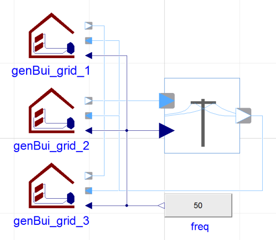
Fig. 10.34 Full simulation test case for 3 grid-connected buildings in Dymola.

Decomposition and graph dependence

Decomposing the model into sub-model for co-simulation is an important question, but it would be far beyond the subject to discuss theoretical aspects. However, in the scope of DES co-simulation through FMI and Modelica models, some good practices and advice can be highlighted. For more details, see also Section 6.7. The model decomposition is usually a trade-off between:

• exchange of quantities that vary slowly in order to use a large communication time step,
• decouple equations to make sub-models simpler to solve,
• create equivalent-size sub-systems to optimize the CPU usage in case of parallel computing.

The Modelica language usually make the decomposition straightforward since it is a component-oriented modeling language that explicitly declares decomposition, inputs and outputs of each sub-components. Moreover, DES typically consist of many similar components that are repeated and linked to each other. As a consequence, one could consider creating communications between clusters of buildings, buildings or, deeper, between heating systems, thermal envelope, and the network. As a starting point, we consider dwellings as several FMUs, and the electrical network as another one.

In our case, on the building side, we consider steady state complex voltage as inputs (supplied by the grid) and current as outputs. After defining the decomposition, one may need to add adapters to convert acausal ports to causal ports such as shown in the code snippet below. This adapter is then used to connect buildings to the grid as shown in Fig. 10.34.

model Pin2FMI_current
"Adapts an acausal connector to input/output signals"

  import QS = Modelica.Electrical.QuasiStationary;

  Modelica.ComplexBlocks.Interfaces.ComplexOutput i;
  Modelica.ComplexBlocks.Interfaces.ComplexInput v;
  Modelica.Blocks.Interfaces.RealInput freq(start=50);
  QS.SinglePhase.Interfaces.PositivePin positivePin;

protected
  QS.SinglePhase.Basic.Ground ground;
  QS.SinglePhase.Sensors.CurrentSensor iSensor;
  QS.SinglePhase.Sources.VariableVoltageSource vSource;

equation
  connect(iSensor.y, i);
  connect(v, vSource.V);
  connect(vSource.f, freq);
  connect(vSource.pin_n, ground.pin);
  connect(iSensor.pin_n, positivePin);
  connect(iSensor.pin_p, vSource.pin_p);

end Pin2FMI_current;

Concerning external resources, on the one hand, weather data should be delegated to a single FMU because of inconsistency risks. On the other hand, occupancy, hot water demand, and all the dwelling-related data could be implemented in the FMU of the associated house. Indeed, those data usually come from stochastic modeling [BS15] and logically differs among dwellings. Three possibilities are available:

1. create one FMU data-reader for all the dwellings,
2. create one FMU data-reader for each dwelling,
3. embed data reading into each FMU-dwellings.

The first solution is straightforward but introduces numerous communications that could affect computation time. Solutions 1 and 2 are not compliant with the boundary condition management of the used IDEAS library in which the information manager is embedded in each building. Therefore, those solutions would have introduced a lot of structural modifications. Embedded data reading in each dwellings implies a specific management of the resources. First, the declaration of all the possible data profiles as resources for each FMU may lead to increased memory requirements. This solution would lead to load all available profiles for each dwelling. Secondly, exporting each dwelling using its own data profile path would be a tedious work, and we thus loose the possibility to change the data profile after the compilation. The solution we developed is to automatically change the resource path during the instantiation of the FMU by casting an integer parameter to the resources’ path as follows:

model GenBui_grid
  "General 2-zone building standalone with dynamic resource path"
[...]

parameter Integer idOcc = 36
"id-number for occupant behavior on external data references";

inner IDEAS.Occupants.Extern.StrobeInfoManager strobe(
FilNam_P="P/P_"+String(idOcc)+".txt",
filDir = Modelica.Utilities.Files.fullPathName("C:/Data/Inputs/"));
[...]

In this example, the resource path points to C:/data/Inputs/P/P_36.txt. This way, the resulting FMU is still generic, i.e. we can change the data profile by changing the tunable parameter idOcc and the instantiation of the FMU would load only one data profile, limiting the memory usage.

The final model dedicated to co-simulation is then a simple combination of FMUs. The dependency graph for 3-connected building is shown on Fig. 10.35.

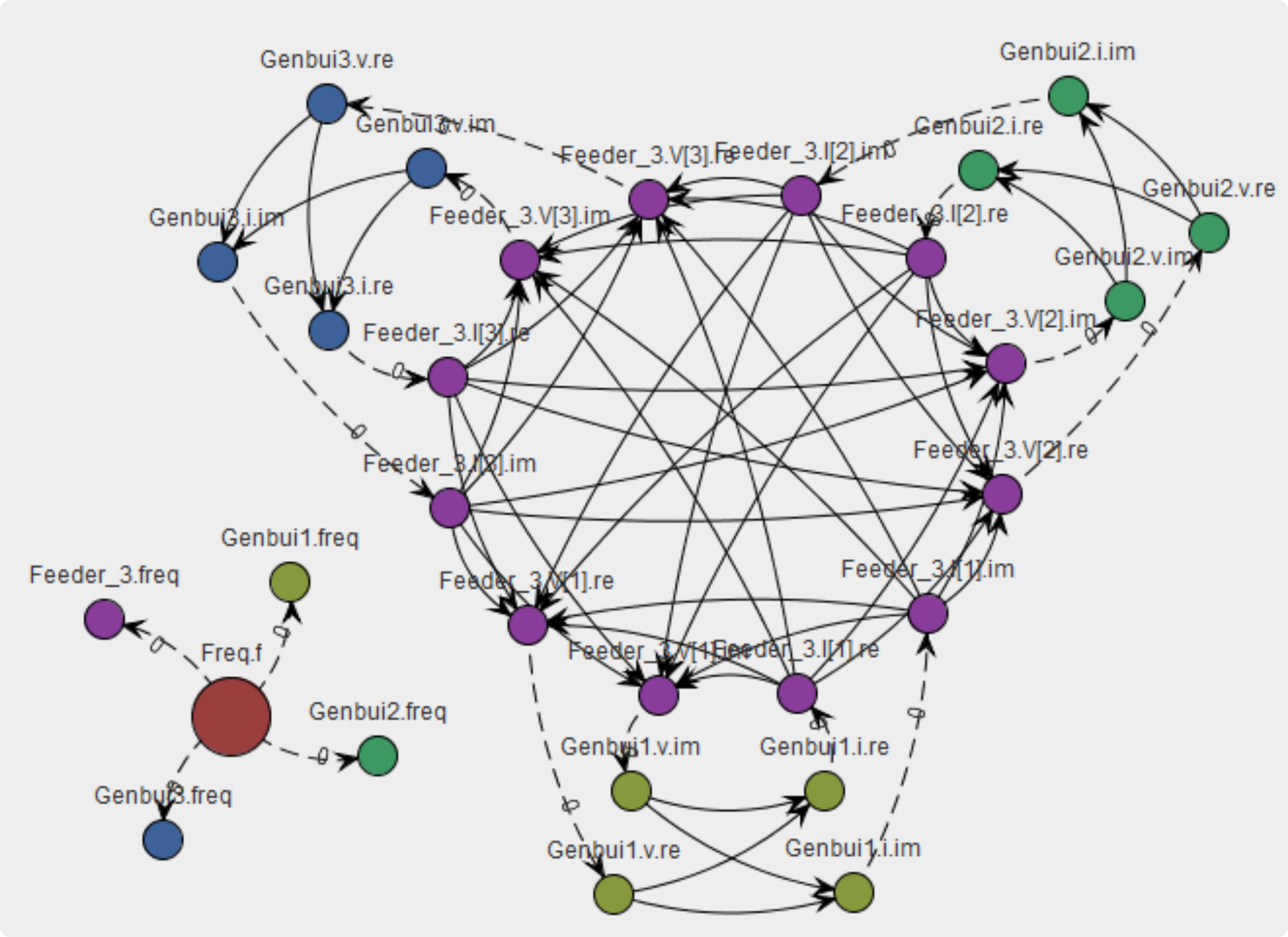
Fig. 10.35 Dependency graph of the 3 grid-connected dwellings.

10.6.2. Computational Experiments

We compared six different simulations for 3 and 6 grid-connected dwellings. This gives us an understanding of the scalability of the simulation. The six simulations reflect changing the solver tolerance, the master algorithm tolerance and the communication time-step in the case of co-simulation. Detailed characteristics of all simulations can be found in Tables 10.3 and 10.4.

Note that the simulation number 6 uses the Daccosim environment and parallel computing [GVD+15] (see Section 6.5.3). Parallel computing using Dymola for simulation and co-simulation shows irrelevant results in term of CPU time and is not reported in this analysis. Only fixed time-step communication was used in the master algorithm.

Table 10.3 Simulations information

Sim.	Environment	Solver tolerance
‘ref’	Dymola	\(1\times 10^{-8}\)
1	Dymola	\(1\times 10^{-6}\)

Table 10.4 Co-simulations information

Co-sim.	Environment	Solver tol.	Master tol.	Communication Time Step (s)
2	Dymola	\(1\times 10^{-6}\)	\(1\times 10^{-6}\)	\(60\)
3	Dymola	\(1\times 10^{-6}\)	\(1\times 10^{-6}\)	\(120\)
4	Dymola	\(1\times 10^{-6}\)	\(1\times 10^{-6}\)	\(300\)
5	Daccosim	\(1\times 10^{-6}\)	\(1\times 10^{-6}\)	\(120\)

Table 10.5 shows the results for the 3 grid-connected buildings, including the CPU time, in absolute format for one year simulation (hour/minutes), in relative format with respect to the reference simulation and the Mean Absolute Error (MAE) of main physical quantities.

One can see that all the co-simulation results are worse in terms of computation time with respect to the complete simulation with the same tolerance (i.e. simulation no. 1). Moreover, MAE for the current might not be acceptable for \(300s\) communication time-step (i.e. simulation no. 4) since it is higher than 2%. We noted that the delay on the voltage is determined by the communication time-step, whereas no delay is noted in the output of the current. This is due to the master-algorithm itself and might be an issue in the context of fast-control and safety, but has no impact on peak or mean values.

Table 10.5 Simulations results for 3 buildings

Sim.	CPU Time	MAE
	(h, min) / ratio	\(I_{re}\)	\(V_{re}\)
‘ref’	\((7, 28)\)
1	\(0.56\)	\(3.12\times 10^{-3}\)	\(1.35\times 10^{-5}\)
2	\(2.18\)	\(5.37\times 10^{-3}\)	\(4.10\times 10^{-5}\)
3	\(1.28\)	\(5.31\times 10^{-3}\)	\(6.36\times 10^{-5}\)
4	\(0.74\)	\(2.04\times 10^{-2}\)	\(1.39\times 10^{-4}\)
5	\(0.78\)	\(5.30\times 10^{-3}\)	\(1.01\times 10^{-4}\)

Note the good accuracy between simulation no. 1 and co-simulation no. 3 and 5 on Fig. 10.36.

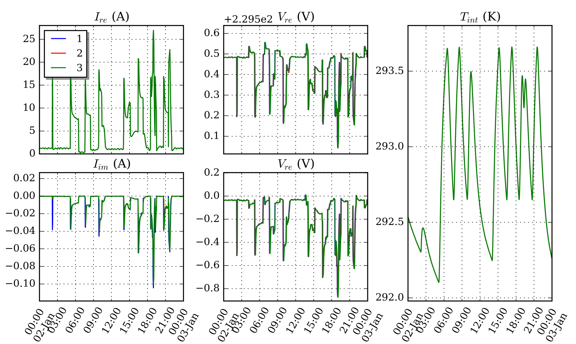
Fig. 10.36 Comparison between simulations no. 1, 3 and 5 : Inner temperature, current and voltage of the building no. 1 for one day.

The results of the 6 grid-connected dwellings are summarized in Table 10.6. Concerning accuracy, the same analysis as the 3-dwellings simulations can be maid, delay on the voltage and a good accuracy for communication time-steps smaller than 300s can be observed. As a result in this case, we consider a communication step higher than 120s not adapted for grid-connected building simulation. However, this value could increase for district heating systems with smoother dynamics.

In terms of computation time, we observe three main results :

1. Without parallel computing, we note lower simulation times due to the co-simualtion itself. The relative computation time decrease from 1.28 (3 grid-connected dwellings) to 0.72 (6 grid-connected dwellings) for simulation no. 3. That means that the gain in computation time increases if the number of buildings is higher. Although, co-simulation no. 3 still is slower than the equivalent simulation, but the gap is decreasing.
2. Doubling the number of connected dwellings increases the simulation time by a factor of 3.45 (i.e. simulations no. 1 and 2), whereas for co-simulation, this factor is about 1.9. This indicates that co-simulation is more scalable and potentially allows increasing the number of buildings in an easier way.
3. Simulation no. 6, using parallel computing, shows the best result with a relative computation time of 0.37, which is even faster than simulation no. 1 using comparable tolerance. Parallel computing on a two physical core CPU divides the computation time by 1.65 to 1.94 compared to an equivalent co-simulation.

Table 10.6 Simulations results for 6 buildings

Sim.	CPU Time	MAE
	(d, h, min) / ratio	\(I_{re}\)	\(V_{re}\)
‘ref’	\((1, 1, 49)\)
1	\(0.56\)	\(2.97\times 10^{-5}\)	\(5.62\times 10^{-7}\)
2	\(1.21\)	\(2.84\times 10^{-3}\)	\(5.13\times 10^{-5}\)
3	\(0.72\)	\(3.33\times 10^{-4}\)	\(9.26\times 10^{-5}\)
4	\(0.41\)	\(1.35\times 10^{-2}\)	\(2.72\times 10^{-4}\)
5	\(0.37\)	\(2.72\times 10^{-4}\)	\(1.23\times 10^{-4}\)

10.6.3. Conclusion and Perspective on Co-Simulation of DES

Conclusion

This section tackled practical aspect of co-simulation of District Energy System using Modelica and FMI decomposition. It involved decomposition and adapting methods for future FMUs and introduced a method to deal with external data inputs using casting to generate heterogeneous occupancy data and save memory during the FMU instantiation. To analyze the possibilities that co-simulation offers, a comparative study involving 3 and 6 grid-connected dwellings, heterogeneous input data, different communication step-size and two environments has been performed. This comparison takes into account the quality of the main outputs, to ensure a good accuracy of results, and the CPU usage. Co-simulation shows a better scalability comparing simulations for 3 and 6 buildings since the computation time was proportional to the number of buildings if used with a fixed time-step communication master algorithm. Moreover, we note a significant time saving using parallel computing. In our experiments, the CPU time was 1.9 faster using a dual-core CPU. Although the speed-up cannot be attributed to the co-simulation methods itself, co-simulation generally facilitates the implementation of parallel computing.

Perspectives

Co-simulation for DES offers many perspectives. From a methodological point of view, one could improve the time simulation considering adaptive communication time-steps. In this case, the scalability of the approach might be decreased. Considering the implementation, parallel computing and an FMU containing inner co-simulation and parallel computing schemes, offers good perspectives in terms of CPU usage and interoperability. From the application point of view, test case using a higher number of buildings could be considered to assess those results for a larger number of dwellings. The effect of the heterogeneity of the structure and the occupancy data profile on the co-simulation performances could be also analyzed for grid-connected dwellings or other DES.

10.7. Conclusions and Outlook

10.7.1. Conclusion

Activity 2.2 “Design of district energy systems” looked into the use of Modelica and co-simulation techniques to analyze DES. The activity consisted of mainly three parts. A first part looked into the existing simulation tools to analyze the behavior of DES. In the second part a common exercise was set-up to develop and test a simple District Energy System and to initiate a framework to develop a validation test called DESTEST. Finally, in the third part of this activity, a preliminary assessment of co-simulation techniques for District Energy Simulations was performed.

Section 10.2 gives a description of all components that enable the delivery of energy services in DES. Because of the research interest of this activity, the focus lies on the modeling of electrical, heating and cooling networks at the neighborhood scale. The literature review of District Energy Simulation models (Section 10.3) focused on Modelica and non-Modelica implementations. It revealed that already many models and tools have been developed for building and district simulations. These models cover a large range, such as building physics, district heating and cooling, electrical network and control. As the analysis of DES requires an integrated whole system approach, often these tools have some drawbacks and shortcomings towards integrated energy system modeling. In many simulation environments, not all domains can be treated at the required level of detail. The many use cases demonstrate the suitability of the Modelica approach to model DES. The following advantages highlight this: numerous available and well-tried models or sub-components can be used to build large scale DES models including multi-physics options that are able to take into account specific phenomena such as bi-directional flows in thermal networks. Modelica is compatible with numerous external simulation environments through FMI exports. The created models can be used as testbed for controllers and as basis to optimize the design and operation of DES.

Section 10.4 reports on the common exercise that has been set up to analyze the capabilities of the Modelica libraries of the Annex 60 participants. It provides a first step to develop a test environment for District Energy Simulations: a DESTEST. A generic Annex 60 Neighborhood Case with 24 buildings was developed. It includes a mix of residential buildings and an office building. The description includes a full description of the building geometry, properties and occupant behavior and defined a heating network and an electricity network connecting all the buildings in the neighborhood. Five Annex 60 participants from different institutions modeled and simulated the heating demand of the neighborhood, using different approaches and Modelica libraries. Surprisingly, the results of the different participants showed deviations for the overall yearly heating demand up to 20% from the average and 15% for the peak heating demand. Exact identification of the cause of the discrepancies was not possible within the time frame of this project. This demonstrates that the many possible modeling approaches and the implementation by different users, each with their own interpretation of the data, indeed may easily result in important deviations.

The purpose of the Annex 60 Neighborhood Case is twofold.

1. It serves as a reference case to analyze relevant research problems such as how to design district heating systems and how to integrate renewables in districts. This was illustrated with two case studies. A first study analyzes to what extent the inclusion of the surroundings in DES simulations influence the result. For the Annex 60 Neighborhood Case, preliminary results showed that taking into account shadowing effects increased the heating demand of buildings with up to 20%. A second study assessed cost-effective retrofit solutions for a DES extension. In both cases, the Annex 60 Neighborhood Case proofed to be useful to execute the analysis.
2. The information and challenges gathered during the development of the DESTEST will be used for setting up a framework to test District Energy System simulation tools. This framework will focus on developing different tests for testing models in a DES context. It also aims to provide benchmarks for academic and industrial analysis for technological solutions, modeling or method assessment.

As an alternative for full Modelica simulations, Section 10.6 analyzed the possibilities that co-simulation of DES using Modelica and FMI decomposition offers. It involved model decomposition and introduced a method to deal with external data inputs using casting to generate heterogeneous occupancy data and save memory during the FMU instantiation. By performing a comparative study involving 3 and 6 grid-connected dwellings, heterogeneous input data, different communication step-size and two environments, it was shown that co-simulation shows better scalability. Furthermore, for the tools used, the co-simulation techniques facilitated the implementation of parallel computing, further decreasing the computation time. Finally, the co-simulation case was an interesting example demonstrating the benefits of the interaction between Activities 1.2 and 2.2 of this Annex.

10.7.2. Outlook

The transition towards zero energy buildings and neighborhoods requires a constant evolution of the tools to design and assess the opportunities and challenge. Already many simulation environments and models exist to simulate the system behavior of the different components that DES consist of. It is expected that this number will rapidly increase and form a comprehensive framework that can be used to design and assess existing and upcoming DES-technologies in a fully integrated and systematic manner. The massive integration of renewable energy sources and reuse of excess energy from buildings and industrial processes demands flexibility in terms of supply and demand. Furthermore, different storage technologies should be added to future intelligent energy systems. In order to adequately apply demand side management techniques and make use of different energy storage options, state-of-the art controllers and algorithms are needed. Future research should look into how to implement these controllers more easily in the simulation environment to test and improve them. Lastly, multi-critria optimization tools should be further improved to facilitate the automated design of DES.

The implementation of data into DES simulation software is often a very elaborate and error-prone process. Moreover, the necessary data are often hard to find or even completely lacking. In short, there is a need for methods to easily implement existing data and reliable data to construct models of existing neighborhoods and to construct representative data sets for a generic analysis. To easily implement real neighborhoods, existing technologies such as BIM and GIS applications have to be further exploited and transformed into a toolchain capable of an automated generation of neighborhoods models. Especially challenging is finding reliable manners to implement missing data. Once such an automated toolchain is developed, it can be used to statistically analyze many different neighborhoods and even cities to create relevant reference neighborhood cases with statistically realistic behavior which is one of the aims of the DESTEST framework continuation in IBPSA Project 1. The question however remains how to verify the results of such neighborhood models. Still, only a limited amount of high quality measurement data are available to perform validation tests. The availability of such a toolchain will facilitate the development of neighborhood models, but will inevitably further increase the computation time and raise scalability issues. This emphasizes the importance of further analysis and development of numerical solvers, co-simulation techniques and parallel computing algorithms.