8. Activity 1.4: Workflow Automation Tools
8.1. Introduction and Motivation
Today, workflow automation tools play an important role in the scope of building and community energy performance simulation as models, tools and engineering tasks become incleasingly complex. Running a script in order to start tools in batch mode and to preprocess variables is common practize in simulation. This is especially true if, for example, multiple domains are coupled, different scenarios shall be investigated, if input parameters are frequently varied, if multiple times a similar task shall be performed or if a conversion of input parameters or data formats becomes necessary. Another issue is that computational capabilities are increasing steadily following Moore’s law. Hence, dealing with simulation models becomes more complex for both, users and developers. Challenges for practitioners in the field of building energy simulations therefore include the handling of bigger amounts of input/output data (many or huge data files) [SN14]. Furthermore, a greater number of simulations will need to be run in order to perform sensitivity or uncertainty analysis of single or multiple parameters [HH11][BJH10]. Analysis of the resulting data by means of visualization or statistical figures [RK11] as well as mathematical operations on the inputs and outputs will increase in importance. The various data formats involved in simulation need to be converted and adjusted in order to allow comparisons and communication between models.
These tasks do not require scientific expertise or any specific engineering skills, rather they are often very time consuming and repeating. If performed multiple times manually, not only valuable time will be wasted, it is also conceived to be error prone and tedious. As a consequence, building simulation researchers should be able to use scripting languages or other automation environments to gain more efficiency while ensuring the quality of their results. According to [SN14] the iterative nature of the building simulation workflow can be leveraged by every step in the process which is automated using Python scripting. Fig. 8.1 is exemplifying the whole simulation process in this context starting from Modelica models based on the Annex 60 Library.
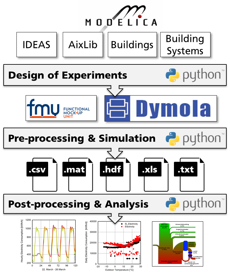
Fig. 8.1 Schematic of typical building simulation workflow to demonstrate use cases for Python based process automation
The importance of workflow automation is also identfied by [SN14] when working with big data. It is recommended to write scripts that automate large batch processes for simulation tasks. Thus, building simulation researchers and practitioners benefit from basic parsing and scripting knowledge.
This chapter provides an overview of associacted Python packages and recommended third party packages. Several Python tools and packages are available for developers and for model users. Those Python tools and packages enhance the workflows for developing and using Modelica and FMI-based models.
They will assist developers in unit tests and checking libraries with conformance to coding guidelines. Furthermore, users will be able to pre-process, run and post-process batches of simulations, such as for parametric studies or for uncertainty propagation, including post-processing of different data formats created by FMUs. It will additionally be possible to integrate Modelica or FMI based models with optimization packages for design optimization and Model Predictive Control.
8.2. Tools and Methodology
This section provides an overview of existing tools and Python packages for automation of building simulation workflows. In the Annex, the necessary capabilities of such tools have been identified and compiled into a common working document. After discussions within the expert groups, a set of mature and utile Python packages was selected, under consideration of their capabilities, license type and implementation language. From the analysis of existing software and features for building simulation automation, a structured list of use cases was derived which reflects the high level requirements for workflow automation tools.
8.2.1. Functional Requirements
The main focus of automation tools lies in the possibility to execute simulations from a script. This is a precondition to efficiently apply pre- and postprocessing functions. These functions are then able to generate the desired efficiency gain for repeatedly used operations. The following paragraph concludes the desired functional requirements of automation tools.
8.2.1.1. Running Simulations
In order to provide a broad foundation for working with simulation inputs and results, the tools should help the user to run different simulation engines like Dymola, OpenModelica, JModelica, FMUs, etc. Simulations of similar types should be processed in parallel. Execution of simulations, especially parametric studies should be done in automated batch setups. An efficient allocation of ressources will be a valuable advantage in this regard. Furthermore, also interaction with external programs in order to couple different simulators is desired. This can also be realized by supporting co-simulation interfaces like the FMI standard.
8.2.1.2. Preprocessing Operations
The initial treatment of simulation input data can be relevant when using changing data sources on the same simulation model, investigating parameter variations or preparing external data for the simulation. In order to support these processes, commonly used scripts should support the transformation of input data (e.g. from BIM data). Also, automated preparation of input data from a database (e.g. product catalogues) is to be considered. This can also be realized based on templates for the simulation model. Parameters for the model can therefore be set instantly. Furthermore, simulation settings, like paths for input data or result files as well as specific simulation parameters (start/end time, verbosity, logging) and solver settings (type, tolerance, integration method) should be handled. Besides the instantiation of parameters, functionality for importing dynamic inputs serving as boundary conditions to the simulation, like specific profiles as data from .xls or .csv files needs to be included. Common data-readers in the Annex60 or other Modelica libraries as well as standardized weather data (TRY, TMY) are only a few valuable input sources to be considered.
8.2.1.3. Postprocessing Operations
Increasing amounts of computational resources, modeling capabilities and memory has led to enormous amounts of data that can be generated from simulations. Automated processing of result files has therefore become a time intensive task. In order to reduce this effort, postprocessing of a set of similar result files, e.g. from a parametric study, must be possible. Furthermore, filtering of result data based on different criteria helps to reduce the data capacity that needs to be handled. However, a suitable way for storing data in larger files or database systems is still necessary, especially when different data sources are to be merged. In addition, computation of typical result criteria like thermal comfort or annual energy consumption needs to be supported.
8.2.1.4. Data Analysis
Gathering parameter sets or patterns of simulation data is often only a first postprocessing step. Various analysis methods, e.g. statistical functions like computing the mean, maximum, minimum or standard deviation of a result variable, can be very useful when analyzing the computed values. More advanced statistical methods involve the computation of a moving average, auto-correlation-functions and ARMA-models. Postprocessing scripts should also be able to compare results with a baseline design option and perform regression analysis such as a linear least square method, trend estimation or curve fitting. The computation of the R² goodness of fit enables fast comparisons between two data series. The ASHRAE Guideline 14 [ASH02] states further values for result interpretation. Besides statistical analysis, frequently used base functionalities for timeseries, like integration, arithmetic or logical operations, as well as frequency analysis, event counting or discarding irrelevent data from a timeseries, can help a user to interpretate and work with simulated data.
8.2.1.5. Data Visualization
Graphical representation of simulation results is a valuable measure to present, compare and analize simulations. Post-processing scripts should therefore inherit typically used options including
- multiple graph plots,
- plot subsets of simulations for comparison,
- various plotting routines for time series, parameter values, box plots, bar charts, carpet plots, scatter plots, histograms, Sankey diagrams, Bode plots or Nyquist plots.
8.2.1.6. Parametrization
Once provided with the opportunity to automatically instantiate and initialize a simulation, methods to execute studies on a single simulation model are necessary. This includes the automated parametrization of models in order to optimize the design. During such a study, often a vast amount of input data is generated and needs to be organized. Sampling methods (e.g. Latin Hypercube Sampling) help to design the experiment (DoE) in order to decrease the data space. A limited number of input parameters are thereby sampled through a probability density function within the design space. The results allow to perform sensitivity analysis and compute uncertainty propagations of the results.
8.2.1.7. Data Conversion
Multiple simulation environments and various data sources lead to the requirement of converting data between different formats. Useful script tools should therefore provide functionalities to handle the container format HDF5, .mos files, tables from .csv and .xls files, .mat files and figures, diagrams as images in .png or .jpg format.
8.2.1.8. Verification
Simulations often serve as supporting measures to better understand a systems behaviour. However, previous verification of such models is important to prevent errors. Automated model check algorithms are therefore a valuable tool to increase productivity. Their functionality should include the verification of model correctness and completeness as well as compliance and model compatibility checking. Furthermore, unit testing can prevent time intensive and cumbersome search for smaller errors in the model. Erroneous input data can be eliminated with fault detection algorithms based on an isolated view of the data itself or in conjunction with test runs of the model.
8.2.1.9. Optimization
After previous simulation generation and analysis, further algorithms can help to support optimization of a system. These incorporate
- derivative-free optimization that evaluates a model for different parameter values; these can be heuristic such as genetic algorithms or particle swarm optimization, or deterministic such as generalized pattern search methods [WW04][PW06],
- gradient based parameter optimization that either numerically approximate derivatives, or that use computer algebra to obtain analytic expressions for derivatives [AGT09].
8.2.2. Associated Packages
The requirements for Activity 1.4 were mapped to existing tools and packages and the missing functionalities and capabilities needed for building simulation tasks (i.e. validation and demonstration) within the scope of Annex 60 were identified. In order to illustrate the advantages arising from these packages, the following ones are highlighted in the example applications.
- BuildingsPy (http://simulationresearch.lbl.gov/modelica/buildingspy/) from LBNL allows for running Modelica simulations in Dymola and inherits functionality to process result files. It furthermore enables unit tests and the refactoring of Modelia libraries.
- awesim from KU Leuven (https://github.com/saroele/awesim) provides functionality to pre- and postprocess Modelica models. It is possible to compile models, set parameters and solver options. Simulations can be run in parallel. Plots based on the result files can be created and filtering of results based on filenames and parameter sets is possible.
- ModelicaRes (http://kdavies4.github.com/ModelicaRes/) is a package to generate simulation scripts for Dymola. Result data can be loaded, analyzed and plotted. The package interacts with the popular pandas package for Python, allowing for numerous statistical analysis.
8.2.3. Third-Party Packages
Other third-party Python packages exist which provide additional capabilities which are useful for the purposes of building performance simulation such as
- DyMat (http://www.j-raedler.de/projects/dymat/), which is a package for handling Dymola’s or OpenModelica’s .mat output files. Browsing for variables and exporting their content to various formats is supported.
- PyFMI (https://pypi.python.org/pypi/PyFMI) is a framework to incorporate the Functional Mockup Interface (FMI) in the Python environment. Functional Mockup Units can be loaded, instantiated, simulated and modified or queried using the provided functions by the standard.
- matplotlib (http://matplotlib.org/) serves to plot and visualize data of various kind. Several graph types can be generated and saved in different formats like .png or .jpg.
- scipy (http://www.scipy.org/) is a package for scientific computing (based on numpy). It includes functionalities imitating Matlab-like treatment of data in the Python environment.
- pandas (http://pandas.pydata.org) is a package for data and time series analysis (similar to the statistics tool ‘R’). Huge amounts of data can be efficiently stored, queried and analyzed in data frames.
- StatsModels (http://statsmodels.sourceforge.net/) includes statistical methods (similar to ‘R’) that allow for statistical tests, intensive data exploration and the generation of statistical models in Python.
- pyTables (http://www.pytables.org) serves to manage hierarchical datasets. Huge amounts of data can be handled efficiently and easily. The package is based on the HDF5 library.
- pysimulator (https://github.com/PySimulator (LGPL)) is a simulation and analysis environment for Functional Mockup Units and Modelica models in Python.
8.3. Examples of Application
The following examples cover some of the previously stated requirements through self-explaining Python code. The IPython Notebook was chosen to serve as the implementation platform of these examples. A Notebook is an interactive Python computing environment that enables users to author workflow automation scripts that include executable code, interactive graphs and plots, textual comments, images and governing equations.
While executing a Notebook it generates output from the executed Pyhton kernel that is running in the background. The multi-media output is fully embedded in the notebook giving a complete and comprehensible record of a computation.
The sequential reading, executing and verifying of computation results in a step-by-step walkthrough facilitates productive and re-usable code for either, model developers and users.
These Notebooks can as well be published as interactive web application (see http://jupyter.readthedocs.io).
Notebook documents available from a public URL (e.g. on GitHub) can be shared via nbviewer.
A web service ist loading it from the URL and displays the Notebook as static web page to be shared with others.
The Notebooks created for the Annex 60 project start with a short description of their purpose, the used packages and the used simulation model as far as it is relevant to fully understand the Notebook. The simulation models are identical or slightly adapted examples from the Dymola libraries involved in the project scope. Within the Notebooks, code cells are bundled to execute specific tasks. Short text descriptions before and comments in the code help to get a clear picture of these fragments. Some of the cells produce output like graphs, dataframes or pure text. These are shown directly beneath the code cells. The requirements for the notebooks to work are the following:
- all used Python packages must be installed. These include the following: numpy, os, BuildingsPy, pandas, pyDOE, ModelicaRes, pyFMI, csv and datetime;
- the FMI library must be installed and set as a system environment variable in order for pyFMI to be able to call FMI functions;
- the path to the executable of the used Dymola version needs to be included in the path system environment variables.
8.3.1. Single Simulation of a Building using BuildingsPy
Running simulations from script can proof beneficial when applying identical pre- and postprocessing patterns to a single simulation. Especially the effort for statistical and graphical evaluation of the results can be significantly reduced. In this IPython Notebook, a framework including relevant function calls to adress these issues for a single simulation in Dymola is provided. In particular, the Python library BuildingsPy is used, supplemented with elements from pandas and NumPy. The model serving as an example in this case is a slightly modified version of the Annex60.Fluid.Examples.SimpleHouse. It consists of a simplified building envelope, a ventilation system including heat recovery and a heating loop with a radiator. In order to start the process, some basic information such as model name, its location as well as the folder for the result files need to be defined. In order for Dymola to compute the model autonomously, a path to relevant packages is defined.
import os

model = "SimpleHouse"
resultFile = "SimpleHouse"

model_dir = os.getcwd()+"\Resources\Examples\SimpleHouse"
resultFile_dir = os.getcwd()+"\Resources\Results_Nb1"
# set directory to dymola libraries
libs_dir = os.getcwd()+"\Resources"

os.chdir(model_dir)
8.3.1.1. Preprocessing
Prior to the simulation run, various settings can be customized. These involve simple parameters like start and stop time of the simulation as well as the desired time step. In addition to that, preprocessing statements and solver settings are given. Finally the simulation is started.
from buildingspy.simulate.Simulator import Simulator

t_start = 0
t_end = 86400*1
h_step = 60

s = Simulator(model, "dymola", packagePath=libs_dir)
s.setStartTime(t_start)
s.setStopTime(t_end)
n = (t_end-t_start)/h_step
s.setNumberOfIntervals(n)
# kills the process if it does not finish after 600 seconds
s.setTimeOut(600)
s.setSolver('dassl')
s.addPreProcessingStatement("Evaluate:=true;")
s.printModelAndTime()
s.setResultFile(resultFile)
s.setOutputDirectory(resultFile_dir)
s.simulate()

Model name       = SimpleHouse
Output directory = .
Time             = Thu Jun 02 12:08:13 2016
8.3.1.2. Postprocessing
A reader object from BuildingsPy serves to retrieve the values of defined result variables and saves them into the IPython workspace as a pandas dataframe. Since the Dymola simulation yields an irregular time grid, an interpolation is performed to match the result values to the above defined timestep. Finally, the results are exported to a .csv file to ensure the possibility of further, individual analysis.
from buildingspy.io.outputfile import Reader
from buildingspy.io.postprocess import Plotter
import pandas as pd
import numpy as np

# variable names to be extracted from the result file are
# determined
variables = ['zone.T','Q_heating']

r = Reader(resultFile_dir+"\"+resultFile, "dymola")
# the original time grid is defined
tSup = np.linspace(t_start, t_end, h_step)
ResultValues = pd.DataFrame(columns=['time']+variables)
for var in variables:
    (time,temp) = r.values(var)
    # results are reduced to the original time grid
    ResultValues[var] = Plotter.interpolate(tSup,
                                            time,
                                            temp)
ResultValues['time'] = tSup
ResultValues.to_csv(resultFile_dir+"\"+resultFile+".csv")
print ResultValues.head()

          time      zone.T    Q_heating
0     0.000000  293.149994     0.000000
1  1464.406780  293.889343  1380.513502
2  2928.813559  294.936695  1840.707414
3  4393.220339  295.025860   702.443914
4  5857.627119  294.288450   241.524324
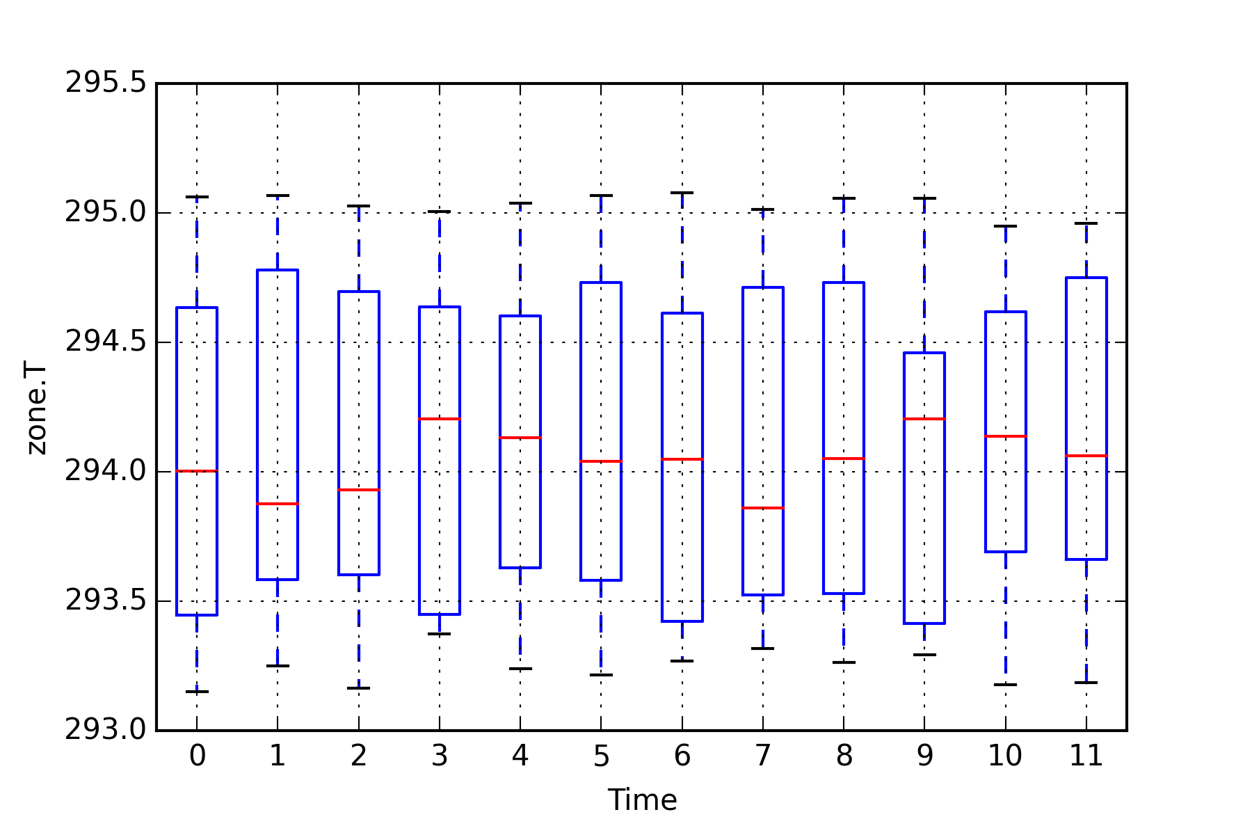
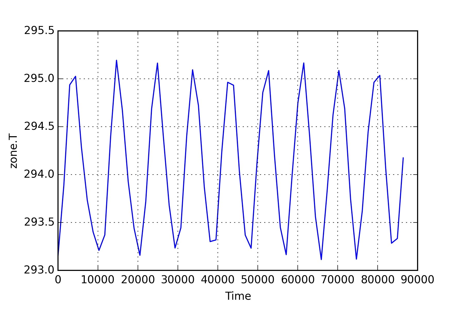
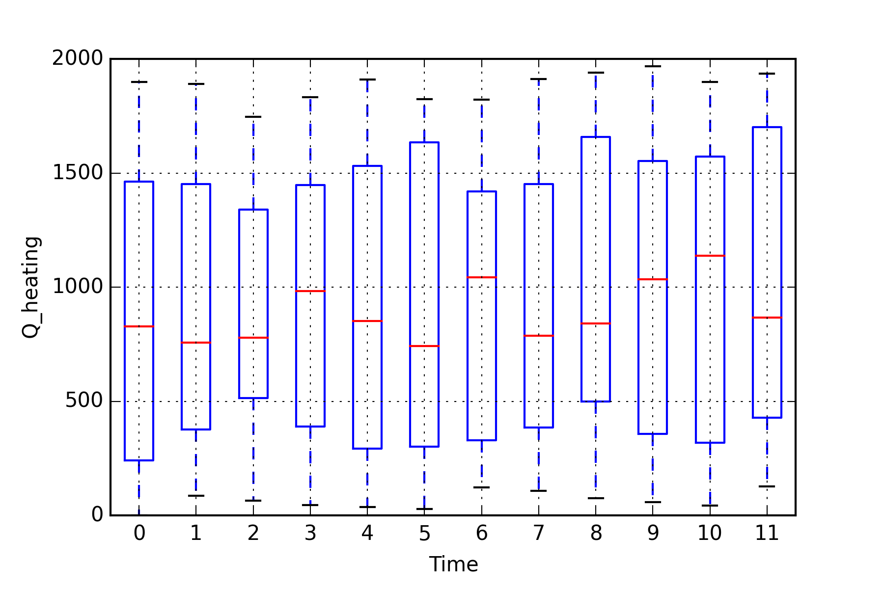
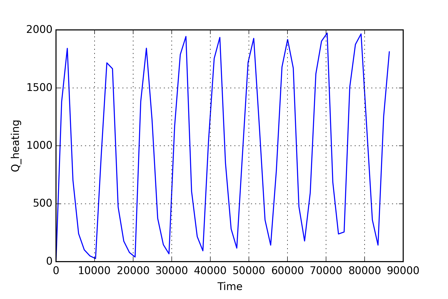
The above defined variable outputs are visualized in two ways using plotting functions from BuildingsPy. The first plot is a boxplot. To execute the function, a time interval needs to be provided over which the boxplot is to be computed. Furthermore, the number of evaluations of the boxplot must be stated. The result is a figure consisting of various boxplots, each representing the given time intervall in sequential order. A second graph produces a simple line plot with the result values represented over the simulation time. Formatting functions provided by the matplotlib can be used within the BuildingsPy package to customize the appearance of the graphs.
for var in variables:

    # 12 statistical evaluations for 600s time intervals.
    # In this case, one hour is divided into 5 minute
    # intervals. For each interval the statistics
    # to create a boxplot are computed.
    plt=Plotter.boxplot(t=list(ResultValues['time']),
                        y=list(ResultValues[var]),
                        increment=600,
                        nIncrement=12)
    plt.xlabel('Time')
    plt.ylabel(var)
    plt.grid()
    plt.savefig(resultFile_dir+"\"+var+"_boxplot.png",
                dpi=300)
    plt.show()

    # a line plot over the simulation time
    plt.plot(list(ResultValues['time']),
             list(ResultValues[var]))
    plt.xlabel('Time')
    plt.ylabel(var)
    plt.grid()
    plt.savefig(resultFile_dir+"\"+var+"_lineplot.png",
                dpi=300)
    plt.show()
The NumPy package provides several useful functions for simple statistics. The following cell computes various measures of descriptional statistics and saves them to a pandas dataframe. The above applied command can be used again to export the dataframe effortlessly to a .csv file.
ResultStatistics=pd.DataFrame(columns=variables)
for var in variables:
    ResultStatistics.loc['Minimum',var] =
        np.min(ResultValues[var])
    ResultStatistics.loc['Maximum',var] =
        np.max(ResultValues[var])
    ResultStatistics.loc['Mean',var] =
        np.mean(ResultValues[var])
    ResultStatistics.loc['Median',var] =
        np.median(ResultValues[var])
    ResultStatistics.loc['25th percentile',var] =
        np.percentile(ResultValues[var], 25)
    ResultStatistics.loc['50th percentile',var] =
        np.percentile(ResultValues[var], 50)
    ResultStatistics.loc['Standard Deviation',var] =
        np.std(ResultValues[var])
    ResultStatistics.loc['Variance',var] =
        np.var(ResultValues[var])

ResultStatistics.to_csv(resultFile_dir+"\"+resultFile+
        "_statistics.csv")
print ResultStatistics

                       zone.T Q_heating
Minimum              293.1131         0
Maximum              295.1935  1972.613
Mean                 294.0912  941.9056
Median                294.052  881.5341
25th percentile      293.4302   232.922
50th percentile       294.052  881.5341
Standard Deviation  0.6809249  708.8307
Variance            0.4636587  502440.9
Some useful BuildingsPy functions can also help to quickly assess certain performance indicators. In this case, an integral function is applied to the required heating power. As a result, the cumulative heating energy over the simulated time period can be evaluated.
print "Total heating energy sums up to" ,
       r.integral('Q_heating')

Total heating energy sums up to 81547626.5705
8.3.2. Parametric Study using BuildingsPy and ModelicaRes
Single simulations can assist practitioners to better understand and assess a system. However, knowing the influence of parameter variation on the system’s behaviour is crucial for system optimization and provides valuable additional insights. The following script serves to automatically run such a parameter study in Dymola based on a Latin Hypercube Sampling (LHS) of chosen variables. The package pyDOE is used to generate the sample for the study. The setup and start of the simulation is executed with BuildingsPy. ModelicaRes is used to label and compare the simulation runs graphically. The modified version of the Annex60.Fluid.Examples.SimpleHouse example is again taken to demonstrate the procedure. Parameters under investigation are the outside wall area of the building, its mean U-value as well as the nominal heating power. The study is performed with the purpose to find suitable combinations of the three parameters in oder to ensure comfortable temperatures in the building. In a first step, the usual settings for model name, directories etc. must be defined. Again, the directory containing relevant Modelica libraries for the model needs to be provided.
import os

model = "SimpleHouse"
model_dir = os.getcwd()+"\Resources\Examples\SimpleHouse"
result_dir = os.getcwd()+"\Resources\Results_Nb2"
# set directory to dymola libraries
libs_dir = os.getcwd()+"\Resources"
os.chdir(model_dir)
8.3.2.1. Parameter Sampling
In order to get a set of simulations, each based on different parameter values, the variables in question need to be determined. A minimum and maximum value for each parameter ensures that the samples are amongst the defined range. These values can represent certain constraints or requirements that might occur during planning. To create the sample, the Latin Hypercube Sampling method, implemented in the pyDOE package, is applied. It creates a multidimensional set of parameter values for the batch simulation. Besides the minimum and maximum values of the variables, the number of total simulation runs must be determined. The output of the following code cell shows the created samples in a pandas dataframe.
from pyDOE import *
import numpy as np
import pandas as pd

# Varying parameters in the study
varList = ['A_wall', 'U_wall', 'Q_RadNominal']
MinMax = [(200,300), (0.4,0.8), (1000,3000)]
# Number of simulation runs
n_simulations = 5

# generation of samples with latin hypercube sampling (lhs)
design = lhs(len(varList), samples=n_simulations)
diff = []
mins = []
# the normalized design values are mapped to the parameter
# ranges
for pair in MinMax:
    diff.append(pair[1]-pair[0])
    mins.append(pair[0])

Sample = pd.DataFrame(design*np.array(diff)+np.array(mins),
         columns=varList)
print Sample

       A_wall    U_wall  Q_RadNominal
0  270.708852  0.730839   2151.677135
1  289.948056  0.700511   2313.956082
2  252.777500  0.548079   1369.952720
3  220.802008  0.587404   2900.892276
4  213.898259  0.437846   1661.255155
8.3.2.2. Batch Simulation
To run the created parameter sets in batch mode, the BuildingsPy package is used. It creates a folder for every run in the result directory. Naming follows the enumeration corresponding to the parameter set number. After defining start and end time as well as the timestep, simulations with the updated parameter sets are executed in a loop and saved to the corresponding folders.
from buildingspy.simulate.Simulator import Simulator

t_start = 0
t_end = 86400*15
h_step = 60

for i in range(0, n_simulations):
    parameters = {}
    for var in varList:
        parameters[var] = Sample[var][i]
    s = Simulator(model, 'dymola', packagePath=libs_dir)
    s.setOutputDirectory(result_dir+'\run'+str(i))
    s.addParameters(parameters)
    s.setSolver('dassl')
    s.addPreProcessingStatement("Evaluate:=true;")
    s.setStartTime(t_start)
    s.setStopTime(t_end)
    n = (t_end-t_start)/h_step
    s.setNumberOfIntervals(n)
    s.simulate()
    del s, parameters
8.3.2.3. Batch Postprocessing
In order to retrieve the results from the individual folders, ModelicaRes is used. Every simulation run receives a label. This label can later on be used to differentiate between the result values e.g. in a graph.
from modelicares import SimResList

sims = SimResList(result_dir+"//*//*.mat")

# labelling
i = 0
for sim in sims:
    label = 'run'+str(i)
    i+=1
    sim.label = label
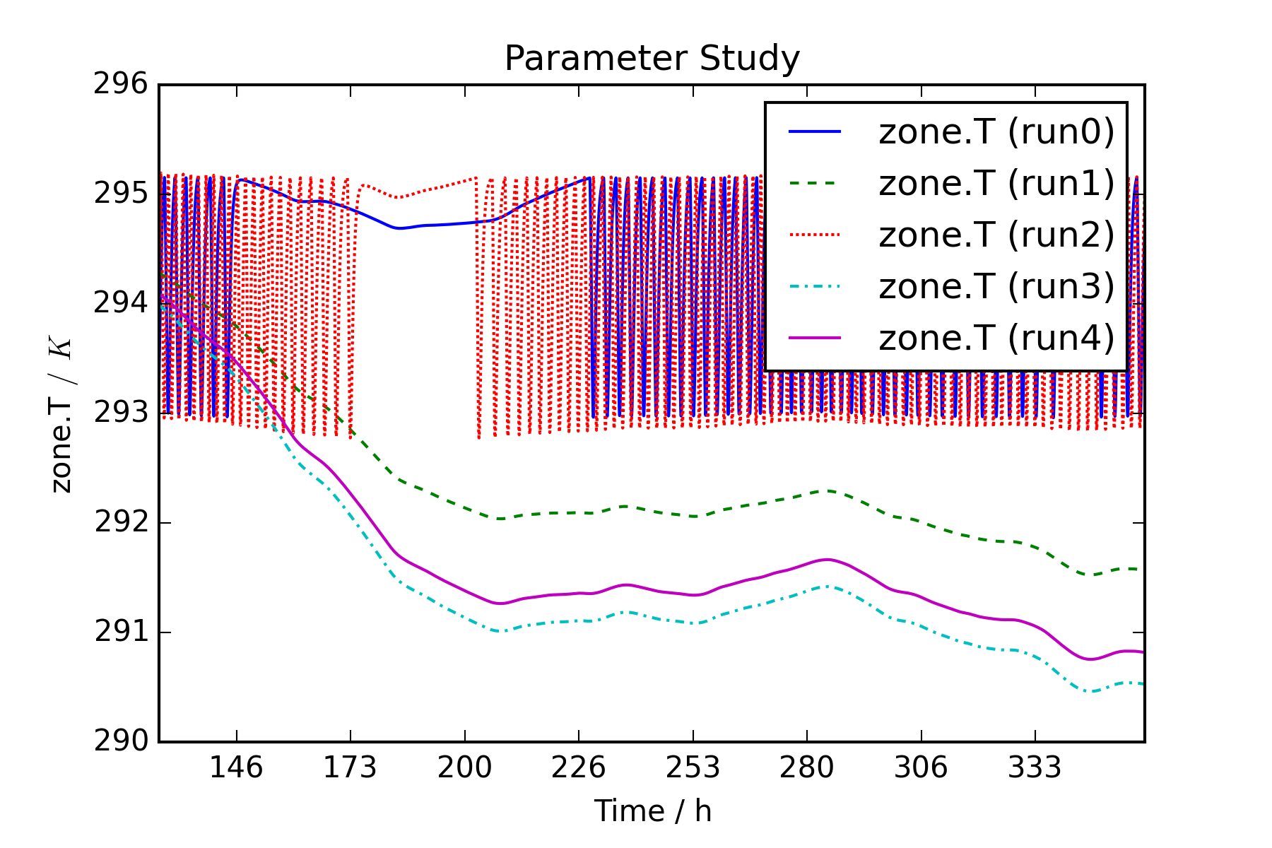
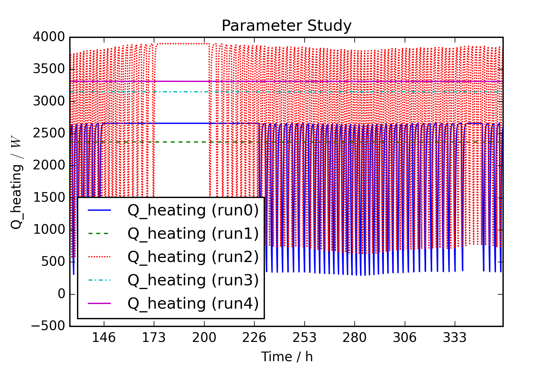
In the following cell, defined outputs of the simulation are compared. ModelicaRes therefore collects the values of each result variable from each simulation run and plots them in one graph. Start and end time of the graph can be provided within the simulation period. The graphs are finally saved to the results directory. Possibilities to customize the graph representation can again be found in the matplotlib documentation.
# define result variables for comparison.
variables = ['zone.T', 'Q_heating']

t_start_plot = 86400*5
t_end_plot = 86400*15

for var in variables:
    fig_temp = sims.plot(ynames1=var, ylabel1=var,
               title="Parameter Study")
    fig = fig_temp[0]
    fig.set_xbound(lower=t_start_plot, upper=t_end_plot)
    labels = fig.get_xticklabels()
    labels_h = []
    for i in range(0, len(labels)):
        labels_h.append((t_start_plot+(t_end_plot-
        t_start_plot)/(len(labels)-1)*i)/3600)
    fig.set_xlabel('Time / h')
    fig.set_xticklabels(labels_h)
    fig.figure.savefig(result_dir+"\"+var+".png", dpi=300)
8.3.3. Parametric Study of a Boiler FMU from Dymola using PyFMI
In certain cases, planners might interact by exchanging simulation models as FMUs for immediate testing of models from other disciplines on design changes. This tutorial on hand shows how to load and run a parametric study of a single FMU exported from Dymola using PyFMI. In this case, the boiler simulation model from the AixLib library is considered as an example. It is a single thermal zone heated by a radiator. The valve between the boiler and the radiator is controlled by a proportional controller. It is the intention to observe the influence of the temperature set point on the total energy consumption of the boiler over a year. To do so, the model is run a few times with different values for the set point.
In order to extract the FMU, this model has been previously compiled in the Dymola environment in the Windows operating system. It is available as the AixLib_Boiler_DymolaWin.fmu file. The PyFMI python package will be used to call the solver and run the simulations. Since the FMU has been exported with Dymola, a Dymola license is needed to run this as well as the following example. Just like in the previous examples, folders and model name must be defined to start with the tutorial.
8.3.3.1. Loading an FMU
from pyfmi import load_fmu
import os

model = 'AixLib_Boiler_DymolaWin.fmu'
model_dir = os.curdir + "//Resources//Examples//Boiler"
result_dir = os.getcwd()+"//Resources//Results_Nb3"
boiler = load_fmu(fmu=model, path=model_dir)
os.chdir(model_dir)
8.3.3.2. Execute Parametric Study in Loop
In the following, parameter values to be applied in the study need to be defined. A loop executes the simulation several times providing the current parameter value as an input signal to the FMU. For each simulation run, the cumulative heating energy is computed in an integral function and saved to a growing list.
from scipy.integrate import trapz
import numpy as np

t_start = 0
t_end = 3.1536e7

T = [291.15, 292.15, 293.15, 294.15, 295.15, 296.15]
Q = []

for TAirSet in T:

    boiler.reset()

    boiler.set('setTemp.k', TAirSet)

    try:
        res = boiler.simulate(start_time=t_start,
                              final_time=t_end)
    except:
        print "One of the simulation cases has failed."

    # The heat flow from the boiler is recovered from the
    # simulation results
    res_time  = res['time']                     # s
    res_Q = res['boiler.heatDemand.Q_flow_out'] # W

    Q.append(trapz(res_Q, res_time) / 3600 / 1000)
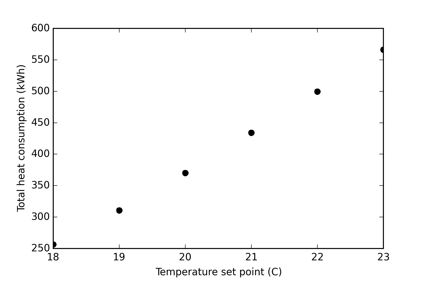
8.3.3.3. Postprocessing
After finishing all simulations, a graphical postprocessing can be started. In this case, a simple point plot is created to demonstrate the dependency of heating energy demand on the temperature setpoint.
import matplotlib.pyplot as plt

plt.figure()
plt.plot([x-273.15 for x in T], Q, 'ok')
plt.xlabel('Temperature set point (C)')
plt.ylabel('Total heat consumption (kWh)')
plt.savefig(result_dir+'\Total heat consumption.png',
            dpi=300)
8.3.4. Import Data to Co-Simulation FMU using PyFMI and Pandas
Input data for simulations can often come from measurements, other simulation results or any external data sources. In order to consider this data in FMU simulations, co-simulation FMUs can be used. Co-simulations offer a step-wise execution of the simulation. After every time step the simulation can be stopped and input values are updated. The package pyFMI offers the necessary function calls to fulfil this purpose. In the following, the SimpleHouse example from above serves as the FMU. In contrary to the original model, weather data is missing in the FMU. Instead, temperature and solar irradiation are read from a .csv file. To start with the notebook the FMU name and its directory must be defined.
import os
from pyfmi import load_fmu

model = "SimpleHouse.fmu"
model_dir = os.getcwd()+"\Resources\Examples\SimpleHouse"

FMU = load_fmu(fmu=model, path=model_dir)
Input and output variables of the FMU can be determined with the following function calls. Later in this script, the found variable names serve as connector to the exchanged weather data.
input_vars = FMU.get_input_list()
print input_vars.keys()

output_vars = FMU.get_output_list()
print output_vars.keys()

['T_amb', 'Irr_HGloHor']
['T_air']
8.3.4.1. Import Tabular Data
A .csv file is imported to IPython in the following cell. The column called “time [s]” is used as a time index. The start date for the time series is chosen in the variable “date”. These formatting measures are necessary in order to be able to map a possibly different time grid of the input data to the time grid of the simulation.
import csv
import numpy as np
import pandas as pd
from datetime import datetime

# Definition of Input .csv file
weatherFile = "Weather.csv"
weatherFile_dir = model_dir

# Data is formated with a time index
date = datetime(2015,1,1)
InputFile = pd.read_csv(weatherFile_dir+'\'+weatherFile)
InputFile.set_index(date+pd.to_timedelta
        (InputFile['time [s]'], unit='s'), inplace=True)

                     time [h]  time [min]  time [s]  T_amb [K]  T_amb [C]  \
time [s]
2015-01-01 00:00:00         0           0         0     278.15          5
2015-01-01 01:00:00         1          60      3600     277.15          4
2015-01-01 02:00:00         2         120      7200     276.15          3
2015-01-01 03:00:00         3         180     10800     275.15          2
2015-01-01 04:00:00         4         240     14400     275.15          2
2015-01-01 05:00:00         5         300     18000     275.15          2
2015-01-01 06:00:00         6         360     21600     274.15          1
2015-01-01 07:00:00         7         420     25200     274.15          1
2015-01-01 08:00:00         8         480     28800     274.15          1
2015-01-01 09:00:00         9         540     32400     274.15          1

                     Irr_HGloHor [W/m2]
time [s]
2015-01-01 00:00:00                   0
2015-01-01 01:00:00                   0
2015-01-01 02:00:00                   0
2015-01-01 03:00:00                   0
2015-01-01 04:00:00                   0
2015-01-01 05:00:00                   0
2015-01-01 06:00:00                 150
2015-01-01 07:00:00                 250
2015-01-01 08:00:00                 300
2015-01-01 09:00:00                 400
After definition of the simulation time grid, the input data can be edited to the given time base. Therefore, the relevant columns of the input file are chosen, resampled and interpolated using pandas. The time indexing within this package is especially practical for this purpose. After preparation of the input data, the FMU co-simulation algorithm can be initialized.
import pandas as pd
from pandas.tseries.offsets import Second

SimInputs = ['T_amb [K]','Irr_HGloHor [W/m2]']

# simulation time grid
t_start = 0
t_end = 86400*1
h_step = 60
t_s = list(np.arange(t_start, t_end+h_step, h_step))

InputVars = pd.DataFrame()
for var in SimInputs:
    InputVars[var] = pd.TimeSeries(data=InputFile[var],
      index=date+pd.to_timedelta(InputFile['time [s]'],
      unit='s')).resample(Second(h_step), how='mean',
      label='right', closed='right')

if InputVars.isnull().values.any():
    InputVars.interpolate(method='time', inplace=True)

print InputVars.head(n=10)

                      T_amb [K]  Irr_HGloHor [W/m2]
time [s]
2015-01-01 00:00:00  278.150000                   0
2015-01-01 00:01:00  278.133333                   0
2015-01-01 00:02:00  278.116667                   0
2015-01-01 00:03:00  278.100000                   0
2015-01-01 00:04:00  278.083333                   0
2015-01-01 00:05:00  278.066667                   0
2015-01-01 00:06:00  278.050000                   0
2015-01-01 00:07:00  278.033333                   0
2015-01-01 00:08:00  278.016667                   0
2015-01-01 00:09:00  278.000000                   0
8.3.4.2. FMU Co-Simulation Algorithm
The co-simulation process requires the exchange of variable values after every time step. In this case, the input variables of the FMU are fed by the imported .csv data. The entire procedure starts with the FMU setup and its initialization. In a loop running through the simulation time grid the following steps are performed. First, the input variables of the FMU are provided with their input values at the corresponding time step. Secondly, the simulation of the current time step is performed. The desired variable results at the computed time step can be retrieved to a pandas dataframe where they are available for postprocessing.
# variable names to retrieve result values from FMU after
# each time step
variables = ['zone.T','Q_heating']

FMU.setup_experiment(start_time=t_start, stop_time=t_end)
FMU.initialize()

ResultValues = pd.DataFrame(columns=variables,
                 index=date +
                   pd.to_timedelta(t_s, unit='s'))

# while loop through simulation steps with i as running
# variable
i=0
while i <= len(t_s)-1:

    # current input values are taken from prepared input
    # file
    T_amb = InputVars['T_amb [K]'][date+
            pd.to_timedelta(t_s[i], unit='s')]
    Irr_HGloHor = InputVars['Irr_HGloHor [W/m2]'][date+
            pd.to_timedelta(t_s[i], unit='s')]

    # Input values from data file are written to FMU inputs
    FMU.set('T_amb', T_amb)
    FMU.set('Irr_HGloHor', Irr_HGloHor)

    try:
        res = FMU.do_step(current_t= t_s[i],
              step_size=h_step, new_step=True)
        if res != 0:
            print "Failed to do step", t_s[i]


    except ValueError:
        raw_input("Error...")

    # variable names defined earlier serve for extracting
    # variable values
    for var in variables:
        ResultValues[var][date+pd.to_timedelta(t_s[i],
            unit='s')] = float(FMU.get(var))

    i+=1
8.4. Summary
Workflow automation is a key tool to automize pre- and postprocessing processes and simulation control in order to perform perform efficient and reliable building performance simulations. Workflow automation is an enabler for massive parameter studies and a precondition as tool for uncertainty and sensitivity analysis and the like. The complexity of systems and associated computational models imposes additional requirements to building researches and simulation engineers. Handling sophisticated building simulations requires basic skills in programming, data processing and statistical analysis. Beginning with a thorough investigation of already existing resources to start from, Activitiy 1.4 compiled and presented useful methods, tools and packages for the aforementioned tasks.
As Python is already established as quasi-standard in the scientific world, it was chosen to be the core scripting language. IPython Notebooks were used as means to present some of the features of existing Python packages in order to assist building simulation engineers and researchers to achieve a higher level of workflow automation.