6. Activity 1.2: Co-simulation and Model Exchange Using the FMI Standard

6.1. Introduction

6.1.1. Motivation for Coupled Simulation

Currently, there is a significant number of sophisticated simulation models and tools available for use in building energy simulation. Models and parametrization are provided by different specialists, with some models being the outcome of many years of development. Hence, different programming languages and modeling approaches are used.

Often, a tool misses functionality provided by others. For many applications it is desirable to use several simulation tools concurrently and make use of results generated by the different models. Consequently, tools running transient simulations often need results generated by other models at runtime. For example, a building energy simulation model computing room air temperatures may require heating loads from an HVAC supply system, with the latter coming from a simulation model external to the building simulation tool.

Pure integration of several existing models into a single simulation tool is technically very difficult, in particular since many tools include their own numerical solver engines and calculation algorithms. Moreover, different simulation tools manage their internal data differently, which further complicates their integration. Also, given different authors, domain experts, copyright limitations, etc. an integration into a single tool may not be meaningful or possible at all. Lastly, future development and maintenance of such an integral model may be difficult to organize. It is also difficult to ensure lasting financial support for development and maintenance of a complex integral simulation tool authored by many individual developers.

Translating existing models into modular equation-based languages such as Modelica could be considered as an alternative, and could benefit from modern Modelica features. Modular, hierarchical design could be used and Modelica tools would be able to optimize the system of resulting equations for performance. However, this approach may not be economically feasible regarding the expected overhead of translating a large number of existing models, and their documentation. Also, copyright and intellectual property protection may not permit integrating their existing model code.

As an alternative, new and existing code of complex systems can be decomposed into sub-systems, the subsystems simulated with the simulator which suits best the specific domain, and interface variables exchanged as the simulation progresses.

Co-simulation is a technique in which simulators are executed simultaneously while exchanging data during run-time. In this context we refer to simulators, also called slaves, as individual component models described by differential algebraic or discrete equations.

The simulators typically embed systems with differential-algebraic equations. Each simulator may implement different numerical techniques tailored to a specific physical or mathematical problem. This includes the possibility that through usage of special programming language features, memory layout, parallelization or other specific optimization, the specialized implementation for model equations may perform better than an equivalent model in a generic simulation environment.

6.1.2. Need for a Tool Coupling Standard

When considering coupled simulation of different tools, several options are available:

1. When access to source code is possible, or tool developers can work actively together, tools may interface directly. Simulation tool developers may even incorporate calculation capability from another tool into their own code. Such a procedure depends on many prerequisites, such as compatible programming languages, proper license agreements, data and calculation structure compatibility and sufficient developer resources. In many cases the resulting code can be considered as a new integrated tool and not really a coupled tool.
2. In the one-to-one approach, two tools implement a specific protocol that regulates exchange of data during runtime. This approach is the most flexible and can support any kind of numerical solution method and also take into account peculiarities of the tools involved. However, the implementation may need to be continuously updated when one of the tools evolves. Also, if tools are developed independently, testing and checking of correct functionality may become time-consuming. Furthermore, interfacing with a third tool typically requires reformulation or adaptation of the protocol and effectively implementing another coupling mechanism tailored to the new tool. Lastly, the development of a clear application programming interface (API) specification and the semantics of the tool coupling is difficult, and subsequent revisions to this API may incur large development costs.
3. To overcome the need for, potentially many, one-to-one exchange protocol implementations a middleware could be used. This acts as a hub for several tools that interface with it and relays communicated data to other connected tools. This approach is less flexible than the one-to-one approach, since a common ground on interface capability needs to be agreed upon. When interfacing domain-specific tools, the middleware can be fitted to the specifics of the problem types and applied numerical methods. Tools need to implement only a single interface and communication protocol and only need to revise code when the middleware is upgraded. However, the same problem regarding the API specification as for the one-to-one approach remains.

In the past, many tool coupling technologies have been developed and applied, with different mathematical concepts and programming interfaces. Many have been tool-specific proprietary interfaces that may change frequently as the original tool developers see fit. Further, the details of interfaces are often restricted to certain applications and lack functionality needed in other physical domains. This is particularly true for domain-specific middleware approaches. In addition, closed-source middleware implementation details may change from version to version, thus potentially render previously connected tools incompatible.

To overcome these limitations it was necessary to develop an open-source and community driven standard for coupled simulation. In 2008 the Modelisar project started to develop such a standard, named the Functional Mockup Interface (FMI, https://www.fmi-standard.org/). Finally, with the initial 1.0 release, a standard for interfacing simulation tools has become available. See [BOA+11] for an introductory paper and https://www.fmi-standard.org/literature for various literature about FMI.

6.1.3. Overview of the FMI Standard

The FMI standard describes the mathematical concept for coupled simulation of several simulators, called Functional Mockup Units (FMU). The FMI standard defines the following:

1. A set of C-functions (FMI functions) that allow exchange of data between FMUs. The standard defines the signature of these function, their required behavior, e.g., the semantics, and it also prescribes during what state of the simulation these functions can or must be called.
2. An XML scheme that is used by each FMU to publish meta-data of the model and the simulator. These data are stored in a file called modelDescription.xml. It contains meta-data such as the number and type of variables to be exchanged and integrated, the capabilities of the simulator, and the mathematical structure the FMU.
3. A zip file with extension fmu that is used to package the XML file, the compiled binaries with the implemented FMI functions, optionally the original source code, as well as resources (databases, project parameters, etc.) required to execute the model.

The FMI standard allows two modes of encapsulating a model: model-exchange and co-simulation. The next sections describe these modes.

6.1.4. Mathematical Aspects of Model Exchange and Co-Simulation

With respect to solving the coupled system of equations arising from all FMUs within one simulation system, two different approaches are standardized. The first, called model exchange, requires a central time integration algorithm that solves collectively the system of differential-algebraic equations defined within the FMUs.

The second approach, called co-simulation, defines a methodology for interconnecting different encapsulated models and numerical solution methods. The individual FMUs incorporate their own integration method that may be tailored towards the physical problem to solve. Also, existing simulator engines can be re-used by implementing a co-simulation interface. The co-simulation master algorithm needs to ensure agreement of all exchanged variables, i.e. that variables computed by one FMU and used by another are correctly synchronized among the tools.

The next sections describe FMI for model exchange and co-simulation, then describe how to synchronize FMUs with a master algorithm, and finally how to generate or export FMUs.

6.1.5. Functional Mockup Interface for Model Exchange

The mathematical concept behind FMI for Model Exchange is based on the idea that a model can be formulated as a function whose output depends on parameters, input variables, state variables and time. Parameters are values that do not change with time. They are assigned at the start of the simulation. Inputs are values that can change with time.

Consider the example illustrated in Fig. 6.1.

Fig. 6.1 Simple room model with air change model and externally defined heat source.

The corresponding Modelica code illustrates the functionality of the model:

model RoomModel
  parameter Real C "Room heat capacity in J/K";
  parameter Real K "Heat loss coefficient in W/K";
  input Real TOut "Outdoor air temperature in K";
  input Real P "Heat added to the room in W";
  output Real Q_flow "Heat exchange with the ambient in W";
  Real T(start=293.15) "Room air temperature in K";
equation
  Q_flow = K * ( TOut - T);
  C * der(T) = Q_flow + P;
end RoomModel;

Suppose now a user wants to incorporate this model into a Model Exchange FMU. The inputs to the model are \(u = (T_{out}, P)\), the state is \(T\), the state derivative is \(dT/dt\), and the requested output is the heat exchange with the ambient \(\dot Q = K \, (T_{out} - T)\). The actual calculation code looks like:

// We have cached the state variable T and
// inputs TOut and P.

// Compute the output.
Q_flow = K * ( TOut - T);
// Compute the time derivative.
dT_dt = (Q_flow + P) / C;

The implementation of the physics of such a model is fairly simple. The model obtains input, caches the state variable and computes the output and time derivative. The time integration will be managed by the simulation master and is not a task of the model. Therefore, no solver to integrate the ordinary differential equation through time needs to be implemented. However, model developers must bear in mind that there is no notion of time step size. Also, the model implementation must not make the assumption that time is always increasing, since the simulation master may request the model to be evaluated several times at the same time, or even requested to go back to a past time instant. See Section 6.1.7 for more detail.

The FMI standard defines a state-machine approach for evaluation of the functions that set inputs, update states, compute outputs, etc. This means, that the model is not evaluated through a single function call passing the complete set of input variables and expecting all outputs and states at once. Instead, the model is treated as an object with a state.

The state of an FMU is only modified when input variables or the time are changed by invoking the FMI functions. While the FMI standard prescribes when the state of the object and outputs are updated, the model can make use of efficient implementation. For example, in our implementation above, if the input P is updated but TOut and T remains unchanged, then Q_flow = K * ( TOut - T) need not be recomputed, saving unnecessary model computation time.

In the model implemented above, all outputs can readily be evaluated without any iteration. However, some FMUs may involve equations that form an algebraic loop. For example, an FMU may implement a hydraulic network which requires an iterative solution to compute pressures and mass flow rate. In this situation, the numerical algorithm to solve such an algebraic loop, typically a Newton-Raphson method, needs to be part of the FMU. Alternatively, the model can be split into two FMUs, and the task of resolving algebraic loops may be delegated to the master algorithm (see Section 6.1.7).

6.1.6. Functional Mockup Interface for Co-Simulation

Co-Simulation describes a calculation method that requires each simulator to integrate its own model equations over a time interval requested by the master algorithm, and exchange outputs only at certain time instants called the communication points. At these communication points, the master algorithm retrieves output variables, and distributes them to other FMUs that use these outputs as inputs. Once the inputs have been updated, the master requests each FMU to integrate to the next communication point. If a simulator cannot advance time to the next communication point, for example because its error would be too large, or because an event happened inside the simulator, it can report this to the master algorithm, which then may request other FMUs to redo their time integration over a shorter time interval.

Co-simulation slaves are, similar to Model Exchange simulators, state objects. The key difference is that for model-exchange, FMUs output the time derivatives of their continuous-time state variables, whereas for co-simulation, FMUs need to integrated this states themselves and output the new values of the state variables.

If the room model example from the previous section is implemented as an FMU for co-simulation, the time integration needs to be performed manually. In the example code below, a simple explicit Euler Integration is implemented:

// We are requested to integrate over the communication
// interval with length h beginning at current time t.

// The FMU state T is stored at time t.
// We have cached the inputs TOut and P at time t
// which are treated constant over the interval t...t+h.

steps = h/dt; // number of integration steps

for (unsigned int i=0; i < steps; ++i) {
  // compute time derivative
  Q_flow = K * ( TOut - T);
  // Update the state
  T = T + dt * ((Q_flow + P) / C);
}

Note that the explicit Euler integration algorithm with fixed time step size may be inefficient. During the time integration from one communication time step to the next, the FMU assumes its inputs to be constant, while in actuality, they may vary more frequently through time. Hence, large communication time steps can incur large errors of the co-simulation.

For example, consider again the thermal room model example above. Suppose the heat added to the room P is computed by a heating system in another FMU. The heater may be controlled by the room temperature and reduce heating power when the set point temperature is approached. The room model provides the room temperature as output. At the beginning of the communication interval, this temperature is passed as input to the heating model, and being below the set point temperature, a heating power is computed. This heating power is then passed to the room model. During the time integration of the room model, this heating power remains constant, and may eventually lead to a room temperature above the set point temperature, as illustrated in Fig. 6.2 [1].

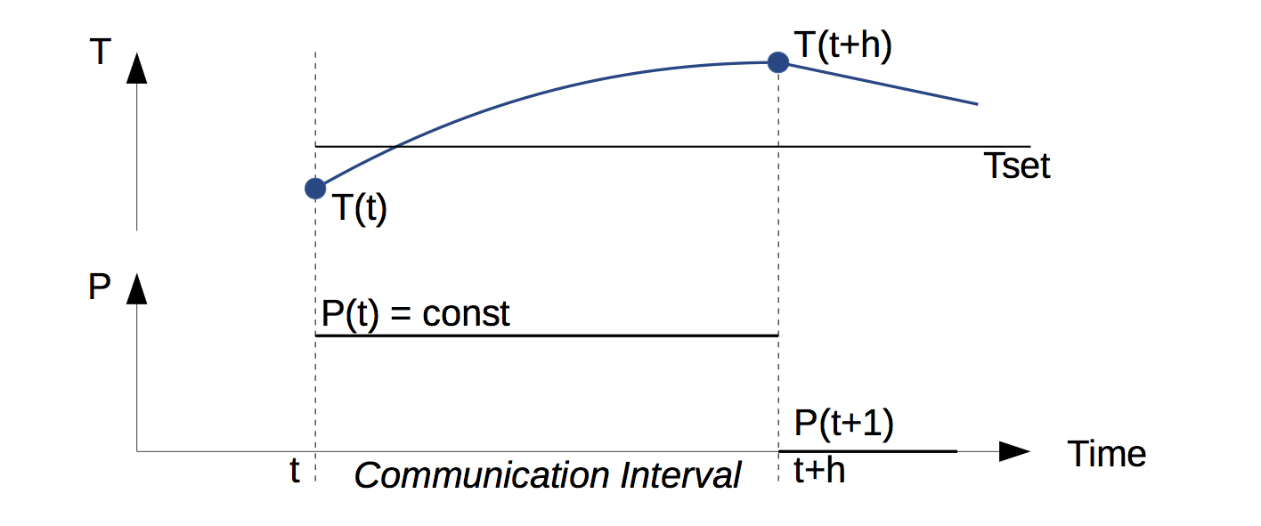
Fig. 6.2 Illustration of room air temperature exceeding the set point temperature due to delayed variable exchange.

While the co-simulation method is a flexible tool coupling approach, it is important to control communication interval sizes and implement suitable algorithms that handle events and control the numerical error of the coupled equations.

6.1.7. Master Algorithms

We will now describe simple master algorithms for model exchange and for co-simulation. Master algorithms synchronize the different FMUs, assign inputs to FMUs, and in the case of model exchange, also provide solvers for differential equations and algebraic equations that are formed by connecting FMUs.

Model exchange master algorithms need to solve systems of differential algebraic equations (DAE). Typically, master algorithms provide different choices for such solvers. When solving the DAEs, the FMU is treated as a mathematical function that computes outputs and time derivatives for given time, inputs and states.

We will now use the FMU example model from Section 6.1.5 to illustrate a simple model exchange master algorithm. An instantiated FMU, named simulation slave, is evaluated in a time integration loop that is the core of the Model Exchange master algorithm. In the following example, an Explicit Euler integration method is used with a predefined number of integration steps:

// ... the FMU slave is instantiated and initialized

// We have stored the initial state of the FMU
// in the variable x.
// The instance m is a pointer to the model.

// Set constant time step sizes based on selected
// steps in the master.
double dt = (t_end - t_start)/steps;

// integrate
for (unsigned int i = 0; i < steps; ++i) {
   // Set new time.
   M_fmi2SetTime(m, t_start + dt * i);
   // Set inputs.
   M_fmi2SetReal(m, ..., &TOut);
   M_fmi2SetReal(m, ..., &P);
   // Set state variables
   M_fmi2SetContinuousStates(m, &T, 1);
   // Retrieve the computed time derivative.
   M_fmi2GetDerivatives(&dT_dt);
   // Integrate in time.
   T = T + dt * dT_dt;
}

In general, a more sophisticated integration algorithm is needed to ensure that the integration error remains below a user-prescribed tolerance, to handle time events and state events, and to integrate the equations more efficiently. Typically, an adaptive time step method is used that adapts the integration time step based on an estimate of the integration error and events. Furthermore, if algebraic loops are present, the master algorithm needs to provide a linear or nonlinear solver. Such algebraic loops are formed if the outputs and inputs of an FMU have direct dependency, and the inputs and outputs with direct dependency are connected with each other.

Implicit time integration methods and nonlinear equation solvers typically use a Newton-Raphson algorithm. Since the Newton-Raphson algorithm builds a Jacobian matrix that has the same dimension as the number of variables, this operation can be computationally expensive. The use of sparse Jacobian matrices is helpful, but requires information on dependencies of individual variables on others. The ability for an FMU to publish such dependency information has been added to the FMI standard in version 2.0. The information about dependency also allows usage of efficient asynchronous numerical time integration algorithms such as Quantized State Systems (QSS) methods [ZL98][Kof03][FK14].

Co-simulation master algorithms assign inputs to outputs of other FMUs, assign the requested time step to FMUs, and advance time of the co-simulation. Hence, each FMU is responsible for integrating in time its continuous-time state variables from the current time to the next communication time point.

Next, we illustrate a basic co-simulation master algorithm with a simple example. Suppose, the room model example above was complemented by a controlled heating model which takes the room air temperature as input and computes the required power of the heating unit based on a temperature setpoint. The heating model and the room model both hold a state at a certain time point. Advancing from this time point to the next communication point can be managed by the co-simulation master algorithm as follows:

// The FMU slaves are instantiated and initialized.
// s1 is the room model, and s2 is the heater model

// Both FMU slaves are at time t and the master algorithm
// has cached the output variables of both slaves.

t = startTime;
h = communicationTimeStep;
// Loop over all slaves.
while(tc < stopTime &&
      status1 == fmi2OK &&
      status2 == fmi2OK)
  // Retrieve outputs.
  s1_fmi2GetReal(s1, ..., 1, &T);
  s2_fmi2GetReal(s2, ..., 1, &P);
  // Set inputs.
  s1_fmi2SetReal(s1, ..., 1, &P);
  s2_fmi2SetReal(s2, ..., 1, &T);
  // Advance time.
  status1 = s1_fmi2DoStep(s1, t, h, fmi2True);
  status2 = s2_fmi2DoStep(s2, t, h, fmi2True);
  // Increment master time.
  t += h;
}

In this example, the master algorithm retrieves outputs, assigns them as inputs to the other FMU, and then requests the FMUs to advance time. Not shown in this example is error handling, as well as handling the situation in which an FMU may reject to advance time to t+h.

The choice of the co-simulation master algorithm can have a great impact on overall performance, as well as on the correctness of the result, in particular in the presence of an event. To ensure that the results of co-simulations of hybrid systems are deterministic and, hence, equal regardless of the tool that implements the master algorithm, [BGL+15] provides requirements and a test suite with expected results that can be used to verify correctness of master algorithms.

6.1.8. Exporting and Importing of Functional Mockup Units

Simulation programs may generate and export FMUs. During FMU export, the simulation model is exposed in such a way that it can be used with the FMI functions for model exchange or co-simulation. The result of the FMU export is a zip file, called the FMU file, as described in Section 6.1.3.

A simulation master or a simulation environment needs to import FMUs in order to use them. Importing FMUs consist of extracting the FMU file, parsing the modelDescription.xml file, and connecting the internal data structure with the FMI functions provided by the FMU. Through these FMI functions, the master or the simulation environment will interact with the model that was provided inside the FMU.

6.2. Use Cases and Applications

Having explained the FMI standard and its philosophy of use, we will now present typical use cases and applications in the design and operation of building and district energy systems in which utilizing FMI offers interesting and innovative perspectives. We will present typical and generic use cases, as well as specific applications that were developed by participants of this activity.

6.2.1. Simulation-Based Building Operation

This use case describes how FMI can be applied to monitor the actual performance of a building relative to the design intent during operation.

During the design, an HVAC designer creates a simulation model of a building, including its HVAC system and controls. The designer then exports the model as an FMU for co-simulation and imports it into a building management system (BMS) such as NiagaraAX. In the BMS, the designer links the model input to measured data. The design model can then be used to compute expected room air temperature or energy consumption, which in turn can be used to compare measured with expected performance. Details of these steps are as follows:

• As a first step, the HVAC engineer develops a model of the building and its HVAC and control system in a modeling language such as Modelica.

• As a second step, the HVAC engineer simulates the building model along with its HVAC and control system to ensure correctness of the control sequence.

  Optionally, to verify the control sequence, the HVAC response and the building response, the model could be decomposed into these three subsystems: Measured data could be fed into the control model to verify actual versus expected control actions; the control signals of the actual system, together with measured outdoor and room conditions could be sent to the HVAC model to verify actual versus expected HVAC efficiency; and the measured HVAC supply conditions and outdoor conditions could be sent to the building model to verify actual versus expected energy provided to the rooms.

• As a third step, the model of the building with its HVAC and control sequence is exported as an FMU for co-simulation and imported into the building management system. The exported system model can then run in real-time to compute the expected performance of the building.

For more information, see [NW14].

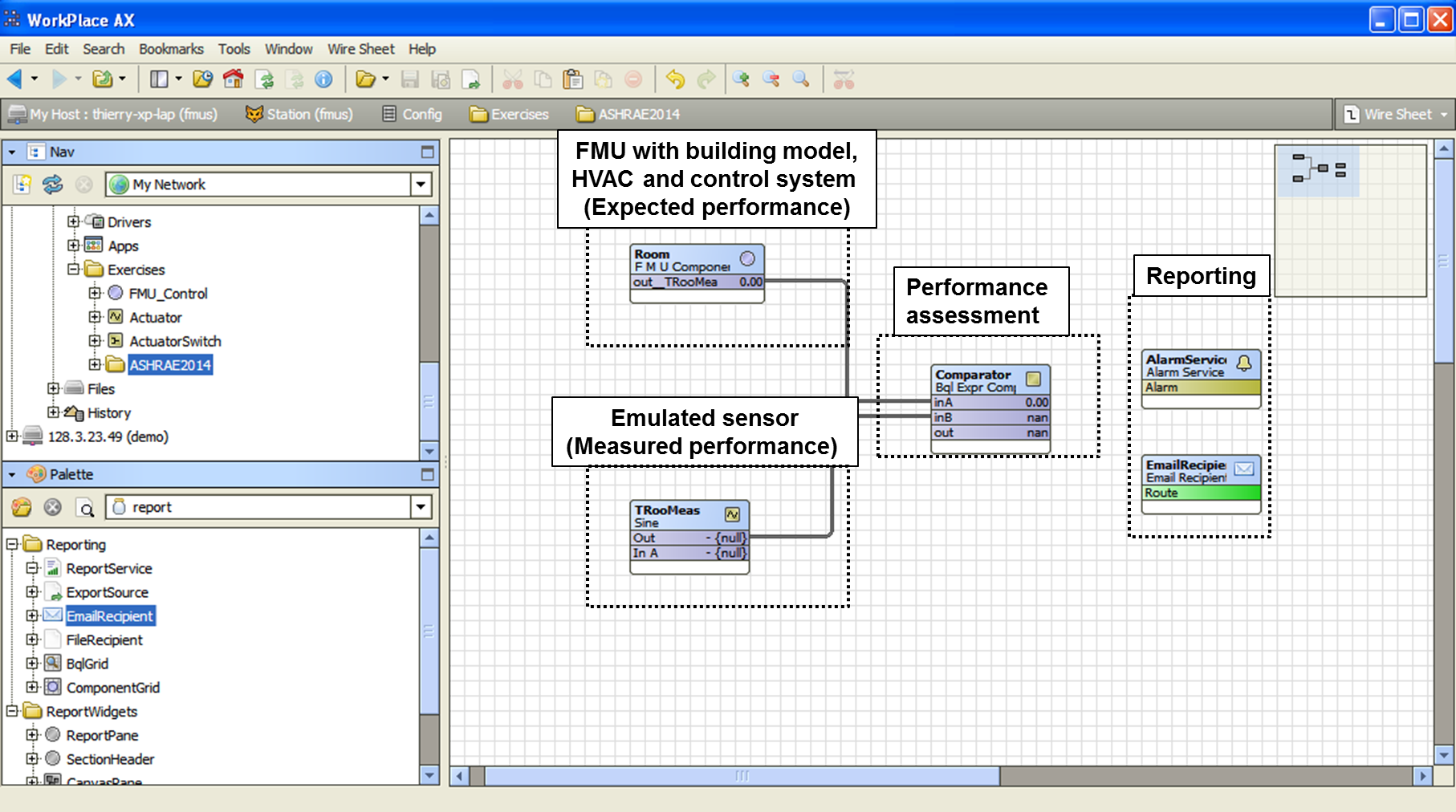
Fig. 6.3 Simulation-based performance monitoring in which an FMU is imported in NiagaraAX.

6.2.2. Design and Operational Analysis of Energy, Control and Communication Grids

Buildings as components of an energy system consume, store and produce energy. In order to provide more global energy efficient solutions and to facilitate the integration of intermittent energy resources, one should consider the interaction of clusters of buildings with the electrical, gas and, if district heating or cooling is present, thermal networks. Such energy grids may have overlying centralized or distributed control, coupled through communication networks.

Such networks are complex systems composed of multi-disciplinary, multi-physics components that can be difficult to handle by any one functional domain: energy assets, information and communication technology and business processes. Energy assets (electrical components, buildings and HVAC systems, industrial processes, thermodynamics) are conveniently described by differential algebraic equations. In other domains, typically for information and communication technology, components are more conveniently expressed by event-based modeling (e.g. representing a market that negotiates energy prices and energy allotments, messaging among distributed equipment, and switching devices).

For such a wide functional scope, a monolithic approach that uses one model with one global solver may require simplified or reduced order models to be computationally tractable. In contrast, distributed simulation, possibly with different numerical solvers for the different domains, is a promising alternative to simulate large systems in parallel. The FMI standard provides a programming interface for models that allows this distributed simulation. Moreover, by encapsulating the domains in FMUs, domain-specific tools may be reused, such as for the simulation of large electrical networks that connect the buildings.

To setup such a distributed simulation, the following four steps are typically done:

1. Generate the models representing the buildings, grid components, control and communication.
2. Export the models as FMUs.
3. Connected the FMUs in a master algorithm, possibly using distributed computing.
4. Control the simulation with a master algorithm.

See also [CBM+16][RGCJ+16] for applications.

6.2.3. Co-Simulation via Domus with Modelica, EnergyPlus and ANSYS CFX

During the IEA Annex 60 project, the research version of Domus, Domus-r, described in Section 6.5.7, has been improved for co-simulation. For EnergyPlus and Modelica, an FMI for co-simulation import interface has been added, while for ANSYS-CFX a script-based interface has been added. In a tool-coupling test case with EnergyPlus, a pure conductive heat transfer envelope model was encapsulated as an FMU for co-simulation and imported into Domus, with the objective to validate the Domus FMI interface.

The Domus pixel counting technique (Fig. 6.4 a) has been used for accurate and fast evaluation of complex shading at internal and external surfaces. The intention of this use case was to simulate the effect that complex shading has on building energy use, with the latter being computed in EnergyPlus.

As a first step of a Domus co-simulation with CFD, Domus has been used to co-simulate with ANSYS-CFX a hollowed block (Fig. 6.4 b) wall. The results are promising and demonstrate a functional integration between Domus and CFX that can expand the current limits of both simulation tools and allow 3-D simulation of building elements.The introduction of the co-simulation in Domus enables detailed, combined consideration of the three heat transfer modes calculated by CFX and integration of this with different tools such as EnergyPlus and Modelica. This would allow for assessment of indoor air quality and building energy efficiency under asymmetric indoor and outdoor boundary conditions. Nevertheless, the high computer run time for CFD is still a considerable constraint so that further research is needed to make it viable.

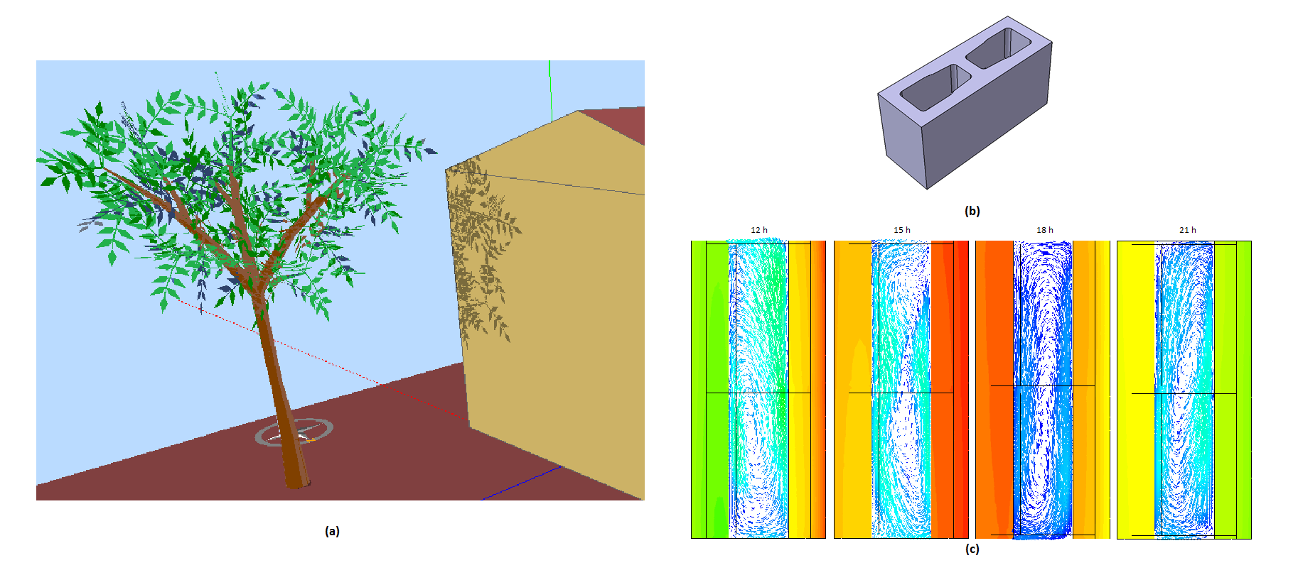
Fig. 6.4 The use of pixel counting technique for accurate and fast evaluation of complex shading (a) at an external surface due to a non-planar tree. (b) The hollowed block used in the wall ANSYS CFX co-simulation and (c) the preliminary results.

6.3. FMI-Compliant Tools for Buildings and District Simulation

This section provides an overview of FMI-compliant simulation tools that are either specifically developed for, or useful for, building simulation. While the majority of these tools have been developed outside of Annex 60, they are listed here to guide new users. A more comprehensive list of those that support the FMI standard can be found on the FMI-Standard website (https://www.fmi-standard.org/tools).

Dymola (http://www.3ds.com/products-services/catia/products/dymola/) is an environment that supports modeling and simulation of multi-physics systems implemented in the Modelica language. Dymola can be used to import and export models as FMUs for both co-simulation and model exchange.

JModelica (http://www.jmodelica.org/) is a Modelica-based open source platform for optimization, simulation and analysis of complex dynamic systems. JModelica has been used by the building simulation community for the simulation and optimization of building energy systems. It supports the export and import for FMUs for model exchange and for co-simulation using the PyFMI Python package.

OpenModelica (https://openmodelica.org/) is an open-source Modelica-based modeling and simulation environment. It has been used in the building community for the modeling and simulation of building energy systems. It supports the export and import for FMUs for both model exchange and co-simulation.

SimulationX (https://www.simulationx.com/) is a modeling and simulation tool which can be used for energy efficiency and HVAC systems modeling and simulation. It supports the export and import of FMUs for both co-simulation and model exchange.

MATLAB/Simulink (http://mathworks.com/products/simulink/) also support FMI import and export using the Modelon FMI toolbox (http://www.modelon.com/products/fmi-toolbox-for-matlab/). A building application case and some implementation comparisons can be found in [WJEP15].

Ptolemy II is an open-source software framework [Pto14] supporting experimentation with actor-oriented design. Actors are software components that execute concurrently and communicate through messages sent via interconnected ports. Ptolemy II has been used to create the Building Controls Virtual Test Bed (BCVTB) [Wet11a]. Ptolemy II supports the import of FMUs which implement FMI 1.0 and 2.0 for co-simulation and model exchange. A large district energy system co-simulation has been implemented in [ZJB+16].

PyFMI (https://pypi.python.org/pypi/PyFMI) is a python package for loading and interfacing with FMUs for co-simulation and model exchange. PyFMI is available as a stand-alone package or as part of the JModelica.org distribution. PyFMI has been used by the building simulation community for applications such as fault detection and diagnostics, and model predictive controls. A building co-simulation example using Dymola models can be found in [RRDW15].

MasterSim (http://mastersim.sourceforge.net) is a co-simulation master algorithm implementation and graphical user interface written in C/C++ (Windows/Mac/Unix) for coupled simulation of FMUs using FMI 2.0. It supports error controlled co-simulation and iterative master algorithms that set and get the state variables.

EnergyPlus (https://energyplus.net/) is a whole building energy simulation program that engineers, architects, and researchers use to model energy consumption for heating, cooling, ventilation, lighting and plug and process loads, as well as water use in buildings. Import and export of model FMUs are available for co-simulation [NWZ14]. Numerous applications can be found in the literature, see for example [DEP16][ZJB+16].

WUFI+ (https://wufi.de/en/software/wufi-plus/) is a hygrothermal whole building simulation program which supports the import of FMUs for co-simulation [PBR+12]. The FMU import functionality was added to integrate Modelica HVAC system models to WUFI.

TRNSYS (http://www.trnsys.com/) is a graphically-based software environment used to simulate the behavior of transient systems. Even though TRNSYS itself does not officially provide FMI support, there is a dedicated FMI-based tool coupling solution openly available at http://trnsys-fmu.sourceforge.net. Furthermore, the feasibility of importing FMUs in TRNSYS through a TRNSYS Type has been demonstrated in [EWP+13][EAWP13].

DIgSILENT PowerFactory (http://www.digsilent.com/) is a state-of-the-art industrial-grade modeling and simulation tool for electrical networks. Even though PowerFactory itself does not officially provide FMI support, it provides several APIs for co-simulation and there is a dedicated FMI-based tool-coupling solution openly available (see http://powerfactory-fmu.sourceforge.net) that utilizes these APIs in an FMI-compliant way.

6.4. FMU Export Facilities

This section describes software packages that can be used to export FMUs and were developed by participants of the Annex 60.

6.4.1. THERAKLES (Room Model)

THERAKLES (http://www.bauklimatik-dresden.de/therakles) is a single-zone hygrothermal model with detailed construction models developed at the Institute for Building Climate Control of the TU Dresden. It includes basic equipment component models. It provides modeling of the thermal storage of the wall by use of spatial discretization techniques. Focusing on deployment in engineering practice, it also provides a user-friendly graphical user interface.

For simulation with more advanced equipment and control logic, the THERAKLES model can be exported as an FMU for model exchange and co-simulation according to the FMI 2.0 standard. A graphical dialog is provided to lead the user through the export process. The generated FMUs provide reset functionality for state variables. Thus, all exported FMUs support error-controlled co-simulation.

THERAKLES has its own climate data base and exports calculated climatic data during simulation. The climate model is encapsulated in the CCM-library which supports an internal binary data format but also reads and converts data from *.epw file format.

6.4.2. NANDRAD (Building Energy Simulation/Multizone)

NANDRAD (http://www.bauklimatik-dresden.de/nandrad) is a building energy simulation framework developed at the Institute for Building Climate Control at TU Dresden. The NANDRAD tool is a command line application designed for the efficient simulation of complex buildings, including detailed wall models. The resulting large differential equation system is solved by state-of-the-art numerical methods, such as Newton-Krylov-iteration methods and sparse matrix algorithms.

NANDRAD supports FMU export for FMI 2.0 co-simulation and model exchange by a script-based automated procedure. The provided input and output interfaces allow the coupling between the NANDRAD building simulation and an external HVAC model, for example a heating or a hydraulic cycle Modelica model. The import of the FMU into a Modelica environment is directly supported by an automatically generated wrapper model. This wrapper encapsulates the NANDRAD FMU, connects all inputs and outputs with vector valued ports and generates a graphical representation. Additionally, NANDRAD precalculates heating and cooling design data and publishes it in a report file.

Similar to THERAKLES, the NANDRAD FMUs support getting and setting of state variables and climate data export.

6.4.3. EnergyplusToFMU

EnergyPlusToFMU (https://github.com/lbl-srg/EnergyplusToFMU) is a software package written in Python that allows users to export the building simulation program EnergyPlus version 8.0 or higher as an FMU for co-simulation using the FMI standard version 1.0. This FMU can then be imported into a variety of simulation programs that can import a FMU for co-simulation. This capability allows, for instance, for modeling the envelope of a building in EnergyPlus, exporting the model as an FMU, and then importing and linking the model with an HVAC system model developed in a system simulation tool such as the Modelica environment Dymola. EnergyPlusToFMU is released under an open-source BSD-license.

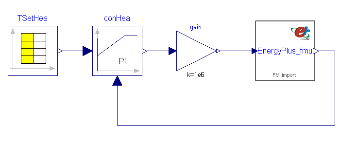
Fig. 6.5 An EnergyPlus room model has been exported as an FMU. This FMU is coupled to a controller implemented in a Modelica simulation environment.

6.4.4. FMI++ TRNSYS FMU Export Utility

Even though TRNSYS itself does not officially provide FMI support, there is a dedicated FMI-based tool coupling solution openly available, called the FMI++ TRNSYS FMU Export Utility. It has been developed using the FMI++ library (see http://fmipp.sourceforge.net/) and enables the export of a TRNSYS model with a Python script as an FMU for co-simulation, using FMI 1.0.

The export tool provides to modelers a special TRNSYS block called Type6139. This type provides external data sent to TRNSYS as inputs to the model and also allows for sending data as external outputs. Apart from the additional input and output block of this type, TRNSYS models are constructed in the usual way as shown in Fig. 6.6.

The FMI++ TRNSYS FMU Export Utility is released under an open-source BSD-license and is available at http://trnsys-fmu.sourceforge.net

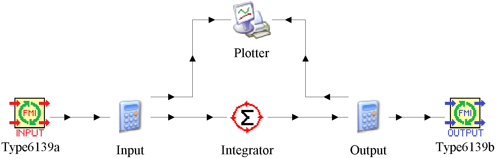
Fig. 6.6 Example of a TRNSYS model containing blocks of Type6139 for FMU export.

6.4.5. FMI++ PowerFactory FMU Export Utility

The FMI++ PowerFactory FMU Export Utility is a stand-alone tool for exporting FMUs for Co-Simulation (FMI Version 1.0) from DIgSILENT PowerFactory models, based on code from the FMI++ library (see http://fmipp.sourceforge.net/). It provides a Python script that creates FMUs from certain PowerFactory models, including the XML model description and shared libraries. Additional files (e.g., time series files) and start values for exported variables can be specified. Currently only steady-state simulations are supported, where the system evolution with respect to time comprises a series of load flow snapshots.

The FMI++ PowerFactory FMU Export Utility is released under an open-source BSD-license, available at http://powerfactory-fmu.sourceforge.net

6.5. Simulation Environments and Master Algorithms for FMI

This section describes simulation environments with FMU import facilities and master algorithms that have been developed by Annex 60 participants. It also describes numerical methods that have been implemented to integrate in time FMUs for model exchange.

6.5.1. Building Controls Virtual Test Bed

The Building Controls Virtual Test Bed (BCVTB) is a free, open-source middleware based on Ptolemy II (http://ptolemy.eecs.berkeley.edu/). It allows users to couple different simulation tools for data exchange during run-time and for real-time simulation. Programs that are linked to the BCVTB are

1. EnergyPlus, the whole building energy simulation program,
2. Dymola, the Modelica modeling and simulation environment,
3. Functional Mock-up Units (FMU) for co-simulation and model-exchange for the Functional Mock-up Interface (FMI) 1.0 and 2.0,
4. MATLAB and Simulink tools for scientific computing,
5. Radiance, the ray-tracing software for lighting analysis,
6. ESP-r, the integrated building energy modeling program,
7. TRNSYS, the system simulation program,
8. BACnet stack, which allows exchanging data with BACnet compliant Building Automation System (BAS),
9. USB-1208LS, the analog/digital interface from Measurement Computing Corporation that can be connected to a USB port.

Fig. 6.7 shows its graphical user interface with a co-simulation model.

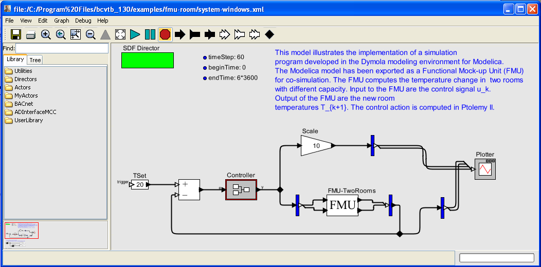
Fig. 6.7 The BCVTB is used to couple a controller implemented in Ptolemy II with a room model implemented in Dymola and exported as an FMU.

The BCVTB has been used in several applications such as agent-based simulation, real-time simulation, control of networked sensors and actuators, and performance prediction of HVAC systems. The BCVTB is released under an open-source BSD license and available at http://simulationresearch.lbl.gov/bcvtb. For more information, see [Wet11a].

6.5.2. EnergyPlus

EnergyPlus (https://energyplus.net/) is a whole building energy simulation program that engineers, architects, and researchers use to model both energy consumption and water use in buildings. To extend the capability of EnergyPlus for building simulation, EnergyPlus has been linked through co-simulation to various programs using direct coupling of tools through custom interfaces and through master algorithms in which EnergyPlus acts as a client.

To address the limitation of these custom coupling mechanisms, an FMI for co-simulation 1.0 import interface has been added to EnergyPlus to support the import of FMUs. Also, a facility has been developed to export EnergyPlus as an FMU for co-simulation 1.0. This interface allows users to link the building envelope of EnergyPlus with an HVAC system modeled in Modelica, or in another simulation tool and language. EnergyPlus is released under an open-source BSD license, and available at https://github.com/NREL/EnergyPlus. For more information, see http://simulationresearch.lbl.gov/fmu/EnergyPlus/export and [NWZ14].

6.5.3. DACCOSIM

DACCOSIM lets you design and execute a simulation composed of multiple FMUs on multi-core computation nodes or distributed on clusters.

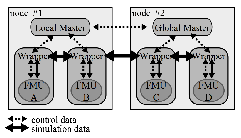
Fig. 6.8 Co-simulation architecture components in DACCOSIM.

A framework is provided to graphically define how the FMUs are connected to each others and on which computation nodes they should be distributed. DACCOSIM automatically generates the associated code and the DACCOSIM library is then used to execute the multi-simulation on the distributed computation nodes. It could be either Java or C++ code.

The main functionalities provided by DACCOSIM are

1. co-initialization with the Newton-Raphson method,
2. inputs extrapolation,
3. support for both constant and variable step size with rollback,
4. various error estimation methods that automatically adjust the step size (Euler, Richardson and Adams-Bashforth),

It runs on Windows and Linux, 32-bits and 64-bits and uses FMI-CS. It is developed by the Supelec IDMaD research team and the EDF R&D MIRE department in the RISEGrid Institute (http://www.supelec.fr/342_p_38091/risegrid-en.html).

DACCOSIM is released under the AGPL open-source license and available at http://daccosim.foundry.supelec.fr/.

6.5.4. Ptolemy II and Quantized State Systems (QSS)

Ptolemy II provides a master algorithm for FMUs for model-exchange and co-simulation, which implements the FMI 2.0 specification.

The master algorithm is implemented in the discrete event domain of Ptolemy II. Additionally, a family of Quantized State System (QSS) integrators is provided to integrate state variables of FMUs for model exchange 2.0. Details about the master algorithm and the QSS integrator can be found in [WNL+15]. The algorithm is release as part of Ptolemy II, and also in the cyber-physical system simulator CyPhySim [LNNW15][BLL+15], which is a subset of Ptolemy II. Both are available under a BSD-license from http://ptolemy.eecs.berkeley.edu/ptolemyII/ and https://chess.eecs.berkeley.edu/cyphysim/.

The CyPhySim simulator supports classical (Runge-Kutta) and quantized-state simulation of ordinary differential equations, modal models (hybrid systems), discrete-event models, the Functional Mockup Interface (FMI) for model-exchange and co-simulation, discrete-time systems, and algebraic loop solvers. CyPhySim provides a graphical editor, an XML file syntax for models, and an open API for programmatic construction of models. It includes an innovation called smooth tokens, which allow for a blend of numerical and symbolic computation, and for certain kinds of system models, dramatically reducing the computation required for simulation. For example, Fig. 6.9 shows a model of a bouncing ball implemented in the CyPhySim simulator. For this problem, a Runge-Kutta 2-3 solver required 14,072 time steps and 3.3 seconds, while QSS required only 46 points in time and completed in 0.085 seconds, or 38 times faster. Furthermore, the QSS solvers have the interesting property that if certain assumptions about the integrator inputs are satisfied, then rollback is never required. If these assumptions are valid, then there is no error due to numerical approximation of the integration, and events such as zero crossings are predictable in advance. For certain cyber-physical systems, such assumptions are indeed valid, and hence computationally exact simulation is possible, where the only source of errors is numerical round-off errors. There is no error due to numerical integration. See [LNNW15] for more details.

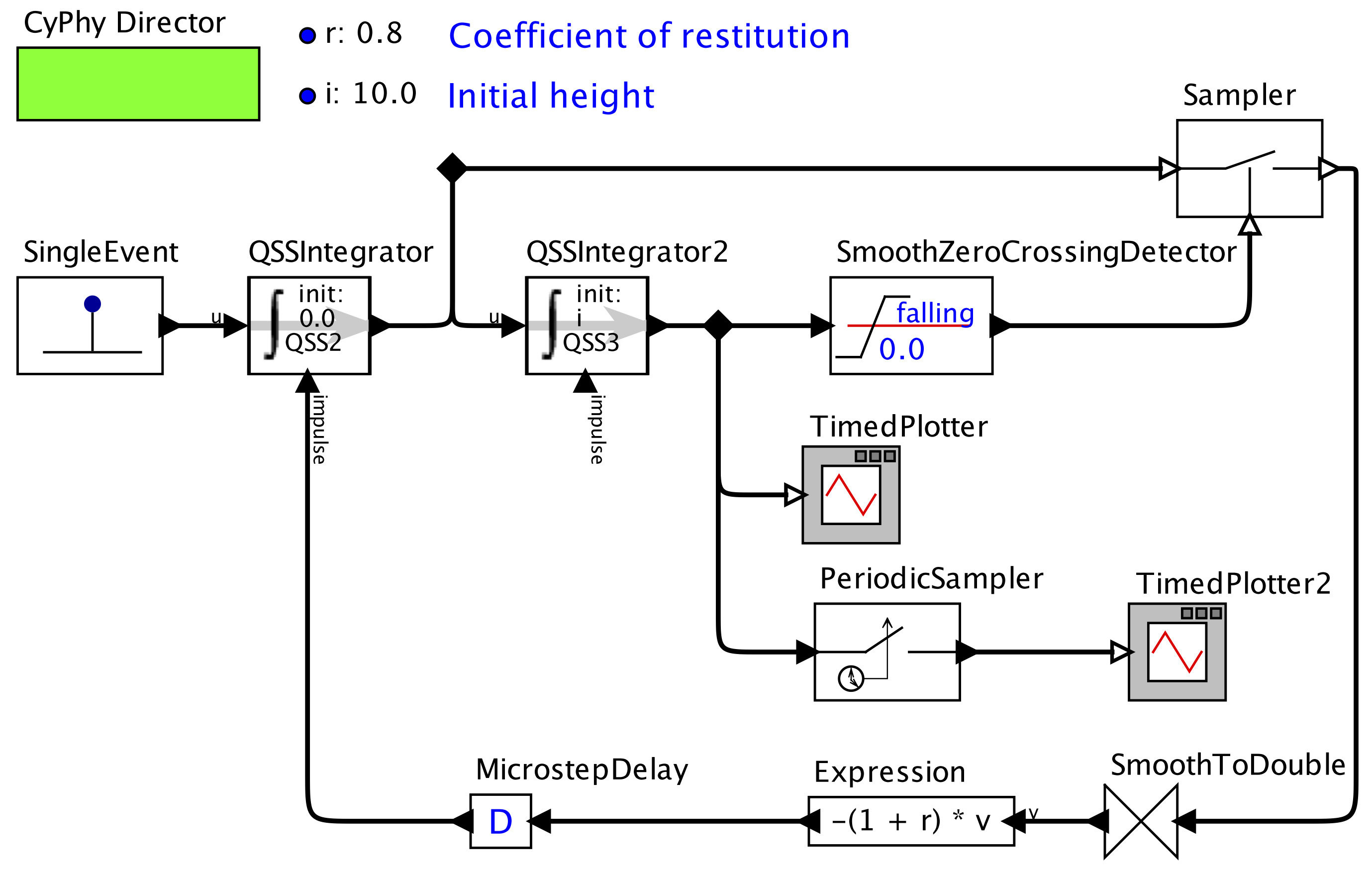
Fig. 6.9 CyPhySim model of a bouncing ball with QSS integration.

6.5.5. FUMOLA - The Functional Mock-Up Laboratory

FUMOLA is a co-simulation framework specifically designed to support the features offered by the FMI specification. FUMOLA is developed on top of the Ptolemy II framework (http://ptolemy.eecs.berkeley.edu/) and the FMI++ library (http://fmipp.sourceforge.net/), mapping Ptolemy II’s functions to the functionality provided by the FMI++ library. Therefore, it provides a flexible platform to investigate the full range of possibilities offered by the FMI specification based on advanced simulation concepts. This allows for implementation of various simulation approaches, including discrete event-based simulations [MW15], simulations of coupled physical systems [WMB+15] and simulations of closed-loop control systems models [WJEP15].

FUMOLA is available at http://fumola.sourceforge.net.

6.5.6. WRM (Waveform Relaxation Method) as a Proposition of a Simple Master Algorithm

The Waveform Relaxation Method [Lel82][LRSV82] has existed since 1982 and was developed and used to solve large systems of ordinary nonlinear differential equations [IC90], in particular for integrated circuit simulations. The method was adapted to be able to be used as a master algorithm for coupling different black box software components such as FMUs [RRDW15].

The idea is to combine several heterogeneous systems that may have different dynamics, and couple them using an iterative method on the waveforms (Fig. 6.10). Each system is solved in time throughout the considered time domain, and its solution, e.g., the entire waveform, is used as an input of the other systems. The procedure can be done for the whole time domain, or for a sequence of sub-domains. This approach is like a strong coupling, and instead of exchanging simple values at a given time, it exchanges the waveform.

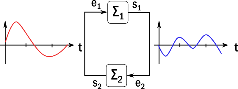
Fig. 6.10 Waveform relaxation algorithm for co-simulation.

WRM has many advantages. The master algorithm is simple and easy to implement. It can be used to couple different components without having to know the internal dynamics and simulation step sizes. In situations where time exchange data between components is important, such as for a web service, the WRM reduces the computation time by reducing the number of calls of the different sub-models. As the simulation time gets longer, the efficiency of the waveform relaxation method increases [RRDW15].

Limitations and disadvantages include less efficient simulations for models that have events. See the application in [RRDW15].

6.5.7. Domus

Domus is a building simulation software written in C++. It has an OpenGL-based graphical interface that has been improved to allow importing models from EnergyPlus 8.0 or higher as a FMU for co-simulation 1.0. Domus has also been improved for

1. shading and sunlit area calculation using a pixel counting technique,
2. reading and writing of EnergyPlus IDF files, and
3. co-simulation with ANSYS-CFD.

This last capability can allow for instance the co-simulation for performance assessment of whole-buildings with 3-D ventilated walls combined with indoor and outdoor air flow under heterogeneous surface boundary conditions. Domus is available from http://www.domus.pucpr.br/. See [MOG03][MBZF08] for more information.

6.5.8. MasterSim

MasterSim is an open-source co-simulation master implementation that supports FMI 1.0 and 2.0.

The simulation master was developed specifically for application in building energy simulation, i.e, interfacing of building simulation models with HVAC system models and control systems, or specialized sub-system models. The master employs several algorithms for obtaining stable, efficient and error controlled solutions. It contains

• different master algorithms/iteration methods, such as non-iterative Gauss-Jacobi, and iterative Gauss-Seidel and Newton methods,
• variable communication step sizes with local error control,
• serialization/deserialization for stop-and-restart of the master.

MasterSim is developed in C++ and runs on Windows, Mac OS X and Linux. Also, the master supports a feature that disables automatic unzipping of FMU archives, which allows for using persistent DLL/shared library files, which is important for FMU developers.

MasterSim is available from http://mastersim.sourceforge.net under a GPL v3.0 license.

6.6. Desired FMI Features and Proposal of Evolutions of the Standard

While the FMI standard is well-suited for our classes of problems, as with any other standard that covers such a complex use case, there are certain limitations encountered and improvements that the Annex 60 participants would like to see in future versions of FMI. As a result of Annex 60, some changes have been proposed to the standards committee. For this cases, we list below the ticket number of the FMI development site. This section provides an overview of the key challenges encountered while using FMI version 1.0 and 2.0, with actions undertaken to address some of the limitations.

Change of array size during initialization: The size of arrays used for inputs, outputs and state variables is fixed once the FMU is generated. It would be desirable to allow defining array variables as quantities where the array size is being controlled by a parameter given during the instantiation of an FMU. This would allow pre-compiling FMUs in which array sizes vary for different applications, such as for CFD, ray-tracing, or heat conduction through solids and through windows.

For this item, the FMI committee has a working group.

FMU time unit: The FMI standard does not specify the unit of the time passed to the FMUs. This can result in synchronization problems if slaves assume a different unit for time. Thus it would be desirable to extend the standard to specify the unit of the time passed to the FMU slaves, or conversely, state in the specification that time is in seconds, which seems to be the implicit assumption and corresponds to what most, if not all, tools implement. Currently, FMU exporters have to agree on a time unit and specify this in the interface description.

A ticket has been filed on the FMI issue tracker (ticket #307).

Handling of FMU-specific output and log files: While FMI 2.0 provides a path to a read-only resource location, such as for data files to be read by the model, it does not provide a path to a writable location where output and log files shall be written. Knowledge of such a writable location is important, for example, when the same FMU is instantiated several times within a co-simulation scenario. Then, each FMU instance needs to use a different root directory for its written files in order to avoid overwriting each other’s files. The same applies when multiple co-simulation runs are executed in parallel using the same FMU files. Hard-coding writable paths inside the FMU does not work in this situation. Use of the current working directory as basis does not work on the Windows platform, since several Windows API function related to file and directory handling change the working directory. The outcome depends on the order in which the FMUs are instantiated and initialized, and on their internal operation. Therefore, it would be meaningful to pass such a directory, if available on the given platform, during instantiation of the FMU. Without a formal method, FMUs must agree on a specific name of the output directory, and the master algorithm must set this before entering the initialization mode of an FMU.

A ticket has been filed on the FMI issue tracker (ticket #299).

Support for structured variables: FMI 2.0 only defines scalar variables in the ModelVariables subsection of fmiModelDescription at the root-level of the schema file modelDescription.xml. Various domains (e.g. fluid, heat transfer, electrical, magnetic, mechanics) would benefit from supporting structured variables of fixed size, especially one-dimensional arrays, instead of only scalar variables. This would also require new fmi2GetXXX and fmi2SetXXX functions.

For this item, the FMI committee has a working group.

Event handling in co-simulation: In FMI for co-simulation 2.0, an FMU cannot announce to the master algorithm an upper bound for the step it can simulate. Rather, an FMU will have to reject a step size requested by the master if it is too long. [BGL+15] suggests a new function fmiGetMaxStepSize that would allow an FMU to announce how long a step it can take. A similar suggestion is also made by [TCT+16], who propose to add the next event time to a new function fmi21DoStep. Announcing the maximum step size would be useful, for example, if a model knows its next time event and hence can ask the master to step no further than that time point. With the current implementation, a master algorithm may step over this time instant, then get notified by the FMU that it went too far, and then ask the FMUs to rollback and do a smaller step.

This item is in discussion within the FMI committee.

Efficient mechanism for output writing in FMI for model exchange: Currently it is unclear how to handle FMU-specific outputs efficiently in FMI 2.0 for model exchange. For example, in a building simulation FMU, at certain time points, usually hourly or every 15 minutes, a lot of output data needs to be stored in output files. Passing that amount of output data through the FMI interface seems not practical.

The integrator within the master algorithm may use a higher-order integration method with variable time steps, such as CVODE. Therefore, integration steps and output steps in the FMU generally do not match.

Currently the only means for the ModelExchange FMU to identify a suitable time point for writing past outputs is the fmi2CompletedIntegratorStep function. The FMU may than write outputs within the last step at the scheduled time point. However, the FMU does not have information about the higher-order integration method of the integrator. Therefore, backward interpolation will likely give different results compared to those computed by the integrator.

A ticket has been filed on the FMI issue tracker (ticket #326).

Master shall be required to set fixed parameters even if unchanged Currently, when specifying fixed parameters in the modelDescription.xml file, the standard does not require that the master calls fmi2SetXXX functions for such parameters. Most master implementations currently set the parameters, even if the values have not been changed by the user.

In order to ensure consistency between the default parameter values set during the export of the FMU and the values in the modelDescription.xml file, it would be useful to require the master to always set the values during the initialization of the FMU.

A ticket has been filed on the FMI issue tracker (ticket #366).

6.7. Best-Practice Recommendations

This section summarizes best practices proposed by Annex 60 participants for building or district-level simulations using the FMI standard.

6.7.1. Climate Data Export

While simulating coupled FMUs, redundant calculations of the same physical part should be avoided because of the risk of inconsistency. Typically, this problem occurs when climate data calculation are performed by different FMUs simultaneously. An example is a system with two FMUs, one for a building model, and one for an HVAC system, which both require outdoor conditions.

As climate data only depend on time, using a common FMU for climate data will not create cyclic dependencies among FMUs.

Since there are different possibilities for defining climate parameters (units, naming conventions, sun coordinate system, etc.) standardizing an interface for climate data would be beneficial.

6.7.2. FMI Interfaces for Room and HVAC Systems

Different variables could be exposed at the interface of rooms and HVAC systems. In order to make different FMUs compatible, an FMI package has been added to the Annex60 library which allows for exporting HVAC models, HVAC systems, and thermal zones as FMUs. This package contains connectors that can be exposed to retrieve and to output HVAC system variables. The package also contains FMI adaptors, which have been added to facilitate the export of HVAC systems. See http://www.iea-annex60.org/releases/modelica/1.0.0/help/Annex60_Fluid_FMI.html for documentation. The rationale for the selection of variables that are used as inputs and outputs of the HVAC FMU are discussed in [WFN15]. Fig. 6.11 shows a model of a heater with the FMI interfaces. The instances bou* convert between causal input and output signals and the acausal fluid ports.

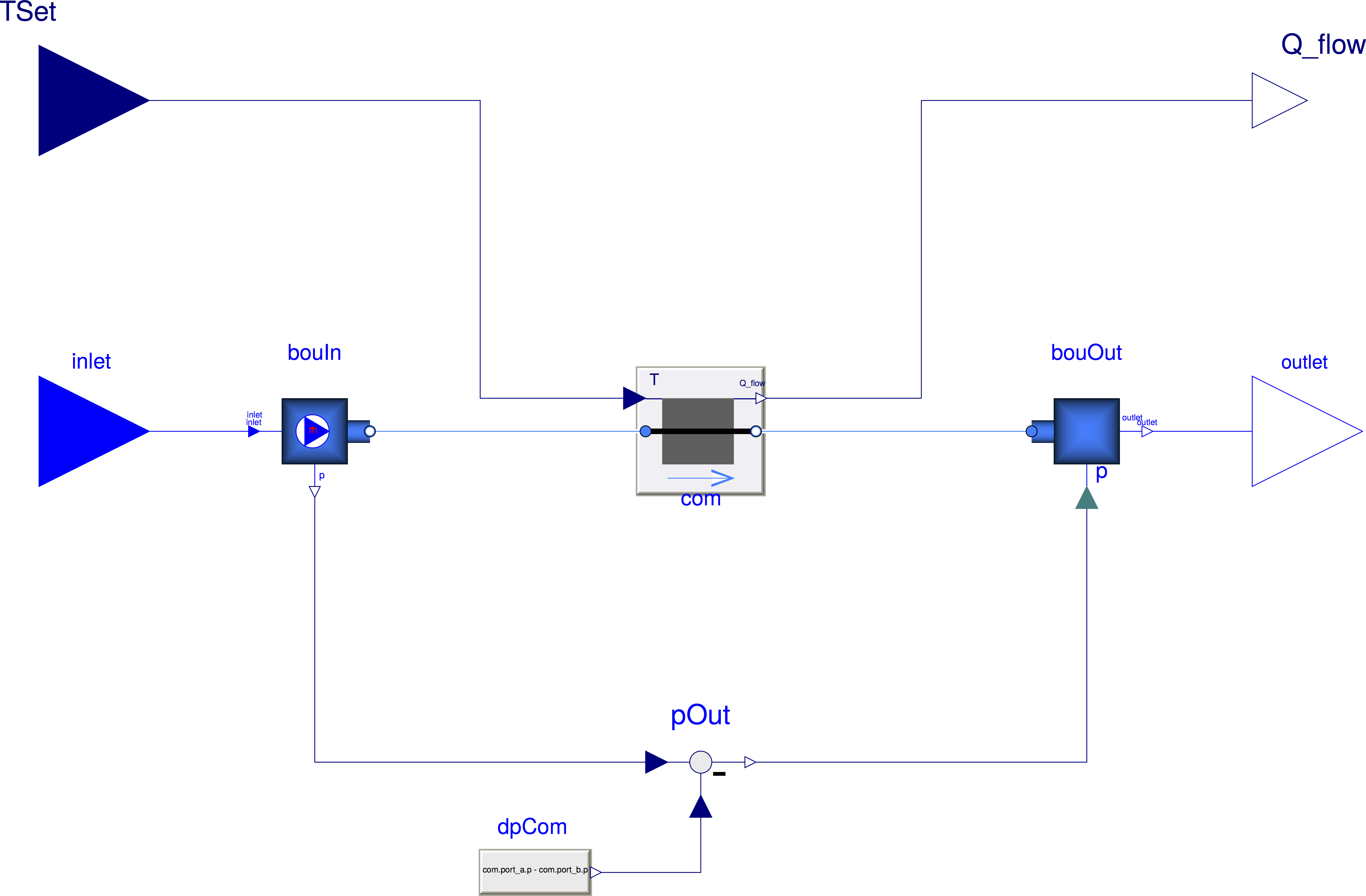
Fig. 6.11 Modelica block that can be used to export a heater that has acausal fluid ports as an FMU.

6.8. Conclusions

This chapter demonstrates that having a standard for exchanging models between different simulators and for linking simulators during run-time is an important topic for building and district energy system simulation. As building and district energy simulation typically involve large models and long simulation periods, having efficient master algorithms is important. The participants of Activity 1.2 demonstrated that FMI is useful for various applications. They also demonstrated the capability of tools to export, import, and co-simulate models encapsulated as FMUs. They showed that the FMI approach is suited for solving the multi-physics, multi-component systems encountered in the simulation of buildings, and they contributed to proposals for further improving the FMI standard. Simulation coupling with open-source standards is potentially a key for tackling the scalability issues that will be encountered for district-level simulations. This is one of the big challenges that building and district energy simulations will encounter in the years to come.

[1]	To allow larger communication time steps, the FMI standard also allows for providing time derivatives of the continuous real inputs.