9. Activity 2.1: Design of Building Systems

This chapter gives an overview about energy-efficient design and optimization of building systems based on the application of Modelica building energy simulation libraries and corresponding optimization methods.

9.1. Introduction

In Activity 2.1, we mean by a building system the combination of the building construction and the corresponding HVAC system. One important advantage of the modeling approach of Modelica is that complex technical systems can be configured in one overall system model. Hence, in the case of the design of building systems, all interdependencies between the thermal building models and the models of the HVAC system can be considered in one coupled numerical problem.

This section is structured as follows:

First, nine case studies are presented in which building energy simulation analysis and building energy designs were performed based on existent Modelica libraries. Second, component models commonly used in these case studies, such as buildings, ducts, pumps and solar collectors, were analyzed to figure out the relevance of the base models of the Annex 60 library. Third, methods for optimal design (OD) and optimal control (OC) for building systems are described and applied in three case studies. Fourth, a Modelica-based building simulation scenario for the exemplary evaluation of OD- and OC-methods is specified. For this purpose, a system model for a solar heating building was developed, which is largely based on the Annex 60 library of Activity 1.1.

9.2. Case Studies

This section describes several case studies, in which Modelica was used to design, analyze and optimize building energy and control systems. Ten different systems of residential and non-residential buildings and their corresponding energy, HVAC and control technologies were modeled by different research institutes.

The description of the different case studies also demonstrates which advantages Modelica offers for building and plant simulation in comparison to other simulation tools and approaches.

The locations of the case studies are distributed over seven countries, namely Germany, Belgium, the Netherlands, Denmark, Iran, Egypt and the USA. Therefore, building energy supply systems both for moderate and for hot climate were evaluated.

The case studies are:

• Development of PV-cooling systems for residential buildings in the MENA region (Section 9.2.1, TU Berlin, UdK Berlin, Germany),
• Control optimization of geothermal heat pump systems combined with thermally activated building systems (Section 9.2.2, Fraunhofer ISE, Germany),
• Investigation of the role of buildings in an European greenhouse gas emission free energy system (Section 9.2.3, KU Leuven, Belgium),
• Implementation of Model Predictive Control for the HVAC system of a Belgian thermally activated office building (Section 9.2.4, KU Leuven, Belgium),
• Modeling for the design of an energy and water efficient hotel (Section 9.2.5, University of Miami, UCI Engineering, USA),
• Design of an innovative two-pipe chilled beam system for both heating and cooling of office buildings (Section 9.2.6, Aalborg University, Denmark and LBNL, USA),
• Integrated optimal design and control of office buildings using renewable energy sources (Section 9.2.7, KU Leuven, Belgium),
• Development of a Virtual Computational Test-bed for Building Integrated Renewable Energy Solutions (Section 9.2.8, TU/e, Netherlands)
• Influence of German energy saving ordinances on heat demand of a residential building (Section 9.2.9, RWTH Aachen, Germany)

9.2.1. Development of PV Cooling Systems for Residential Buildings in the MENA Region

This case study deals with the simulation-based development of PV-cooling systems for residential buildings, located in different countries within the Middle East and North Africa (MENA) region. The hot climate in the MENA region leads to a relevant cooling demand in the summer in residential buildings. The standard used active air-conditioning technologies in the MENA region are water evaporation coolers, often used for dry climate conditions, and also electric-driven small vapor-compression chillers (mostly split units), in particular in regions where natural drinking water resources are scarce (see Fig. 9.1):

Fig. 9.1 Locations of the case study in Iran and Egypt (left) and typical residential building in El Gouna with room-wise installed split unit devices in the facade (right).

As an alternative, the available high solar irradiation potential in the MENA region, for example 1,900 kWh/(m²a) in Hasthgerd New Town (located in the northern part of Iran, 100 km west of Tehran) or 2,400 kWh/(m²a) in El Gouna (located at the coast of the Red Sea, 500 km south of Cairo) can be used to minimize the CO2-emissions by fossil building air-conditioning (see both locations in Fig. 9.1). Within the Young Cities project, different energy concepts for residential building cooling were developed for a new planned 35 ha district in Hashtgerd [HNG11]. One of the proposed technical solutions was a PV-based cooling system, which can store the produced electricity in an electric battery and the cooling energy from the compression chiller in a cold water tank, before it is used for room cooling purposes in a multi-family house with 278 m²net floor area.

Fig. 9.2 illustrates the principle of a PV cooling system for air-conditioning of residential buildings:

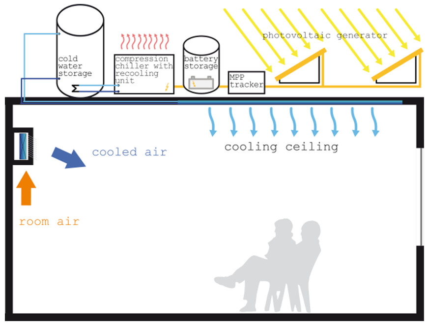
Fig. 9.2 PV cooling system, which supports direct air cooling and indirect surface cooling

The new developed PV cooling system was modeled in Modelica as a base for different simulation analyses for the locations Hashtgerd (North-Iran) and El Gouna (Red Sea, Egypt). The main objectives were the optimization of the energy system design and its most important system parameters, namely the size of the PV-generator, the capacity of the electric battery, the volume of the cold water tank and nominal power of the compression chiller. Furthermore, suited control strategies for the energy management were considered.

A corresponding simulation system model in Modelica is shown in Fig. 9.3:

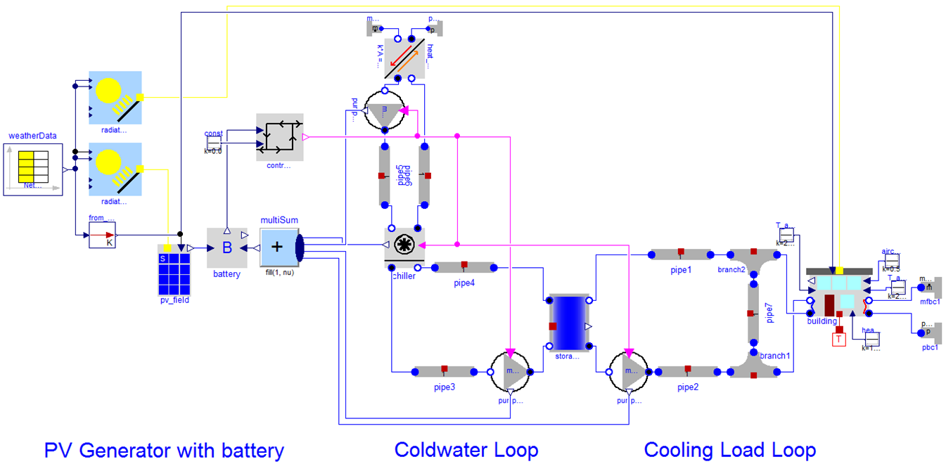
Fig. 9.3 Plant diagram of the PV cooling system, based on the Modelica BuildingSystems library

The model diagram illustrates the different energy transformation steps from the solar irradiation to the generated and stored electricity (PV generator with battery), the cold water production with a compression chiller (cold water loop), the storage in a cold water tank and the use of the cooling energy by the building (cooling load loop).

The system models for the simulation analysis were configured with the component models of the BuildingSystems library [NGHLR12].

The whole energy system was modeled in Modelica and simulated with Dymola. A simplified thermal building model with one zone was used. In a more detailed analysis, a thermal multi-zone building model, modeled in EnergyPlus, was combined with the energy plant model in Modelica. Both sub-models were integrated in a co-simulation, realized with the BCVTB [Wet11a]. For the optimization of the system parameters such as the nominal power of the PV generator or the capacity of the electrical battery, the GenOpt optimization program (http://simulationresearch.lbl.gov/GO/) was used.

9.2.2. Control Optimization of Geothermal Heat Pump Systems Combined with Thermally Activated Building Systems

The simulation analysis focuses on the control optimization of space heating and cooling concepts that utilize environmental energy as heat source and sink. In this study a simulation-based analysis was performed for the inHaus2 located in Duisburg, Germany, as shown in Fig. 9.4. The inHaus2 is a building owned by the Fraunhofer-Gesellschaft for the demonstration and evaluation of building related technologies (http://www.inhaus.fraunhofer.de/en.html). It consists of 3 building segments with a total net useful area of 3,700 m²for laboratory, research, conference and office areas. The heating and cooling energy demand of the building is approximately 60 kWh/(m²a) and 14 kWh/(m²a) respectively.

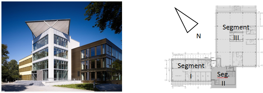
Fig. 9.4 The inHaus2 Building and the orientation of the 3 segments

The space heating and cooling is mainly realized by a heat pump system using near surface geothermal energy with 12 borehole heat exchangers, each with a depth of 120 m. The nominal heating power of the heat pump is 75 kW with a COP of 4.4 at the operating point B0/W35. Mostly thermally activated building systems (TABS) in terms of concrete core activation are used for the heating and cooling of the rooms. Cooling of the building is by means of passive cooling with the borehole heat exchangers and by active cooling using the heat pump as a chiller with a nominal cooling power of 69 kW and an EER of 6.0 at the operating point B35/W18. A monitoring system is installed in the energy supply system for the evaluation of the system performance. The data can also be used for the validation of the simulation models.

Fig. 9.5 shows the HVAC components that are integrated in the energy supply system for heating and cooling of the inHaus2.

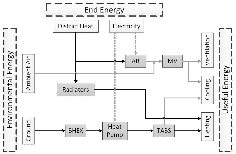
Fig. 9.5 HVAC Schematic of inHaus2: AR-Adsorption Refrigeration, MV-Mechanical Ventilation, BHEX-Borehole Heat Exchanger

The objective of the study was to develop optimized control strategies for the thermal as well as the hydraulic system of the geothermal heat pump system. The thermally activated building systems have a high thermal mass and therefore cause controls difficulties for the room temperature which can lead to over- or under-supply of the thermal zones. Furthermore, the hydraulic heat distribution system causes high energy consumption for the circulating pumps due to the long pipe network and high volume flow rates in the hydraulic circuits for the TABS, as well as the borehole heat exchangers.

It has been observed that the auxiliary energy in such systems can amount up to 30 percent of the total end energy consumption of the building [KH09]. Therefore, this study aimed at a thermo-hydraulic optimization of the control of the whole system concerning minimized end energy consumption under consideration of the thermal comfort requirements of the building.

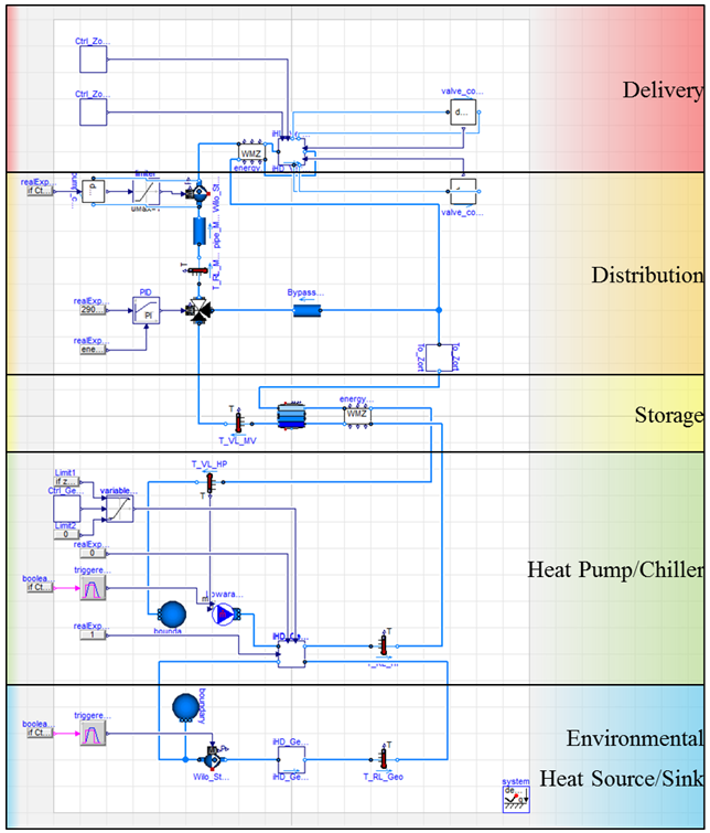
Fig. 9.6 Representation of the geothermal heat pump system of inHaus2 in Modelica

Fig. 9.6 shows the representation of the geothermal heat pump system of the inHaus2 HVAC system in Modelica. The system model for the simulation analysis is built using component models of the Buildings library [WZNP14], the Modelica Standard Library (MSL) and models that are developed at Fraunhofer ISE.

For the optimization analysis, an executable dymosim file and an input file with the initial states and parameter values were generated from the system model in Dymola. Using these files, the optimization was realized with the optimization tool GenOpt (http://simulationresearch.lbl.gov/GO/). The system control optimization also had to take into account predictions for weather and internal heat gains. Therefore, a Python-framework for the realization of a model-based predictive control (MPC) was built, which coupled the system model and the optimization tool GenOpt.

9.2.3. Investigation of the Role of Buildings in an European Greenhouse Gas Emission Free Energy System

This case study was part of a project called “A fundamental study of a greenhouse gas emission free energy system” which studies the European energy system in 2050 assuming that the energy system would be all-electrical. An important part of this project was on the potential of demand-side response of electric vehicles, appliances and heating and cooling of buildings, as shown in Fig. 9.7.

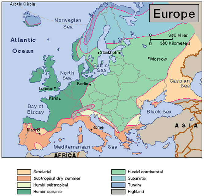
Fig. 9.7 Europe’s building stock will be studied, taking the different climates and current building stock into account. (Source: http://drmrenfrew.files.wordpress.com/2013/08/europe_climate-map-western-europe-atlas.gif)

The study focuses on residential buildings. A large range of technologies was considered, namely these which use local renewable energy sources (such as biomass, solar thermal, PV and geothermal) or electricity (such as heat pumps and electrical resistance heaters), eventually combined with thermal grids.

This study followed a back casting approach. The aim was to determine which combinations of energy technologies in 2050 make it possible to have a greenhouse gas (GHG) emission free energy system. For this purpose, a number of scenarios were simulated. The building stock was represented by a set of simplified models from which the energy demand and the flexibility of this demand were extracted (see Fig. 9.8).

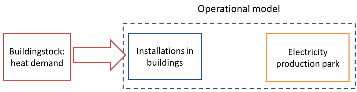
Fig. 9.8 The interaction between the heating and cooling systems in buildings and the electricity production park was studied with an operational model which has information of both systems [Bal13].

The validity of these simple models was checked against detailed models in Modelica. In a later step, optimizations were performed, determining for each scenario what the optimal combination of HVAC systems is. The study ran from October 2011 to October 2015. Fig. 9.9 shows an exemplary system model for the above described approach.

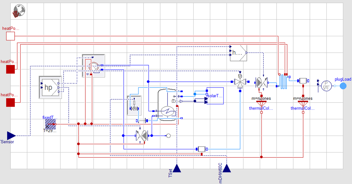
Fig. 9.9 Results of the operational model will be checked with simulations in Modelica using the IDEAS library [BDCVR+12]. This figure is an example taken from the IDEAS library.

The IDEAS library [BDCVR+12] was used for the verification of the simple models used in the operational model. The operational model was implemented in GAMS, using Matlab for pre- and post-processing. The verification of the results were done by performing more detailed simulations in Modelica using Dymola. The second part of the work, namely the optimization of the heating and cooling systems in different scenarios was performed in Matlab by using the yalmip toolbox [Lof04].

9.2.4. Implementation of Model Predictive Control for the HVAC System of a Belgian Thermally Activated Office Building

The case study building, called “Hollandsch Huys” and shown in Fig. 9.10, is located in Hasselt, Belgium. Its construction was finished in 2007. Designed to be a low-energy, innovative office building, it makes use of thermally activated building systems (TABS), in which the thermal mass of the concrete floors is activated by a water piping circuit for both heating and cooling. The heat and cold are produced by a ground-coupled heat pump (22 single-U-tube bore holes of 75 m) and with a gas-fired boiler of 60 kW as back-up for the air handling unit.

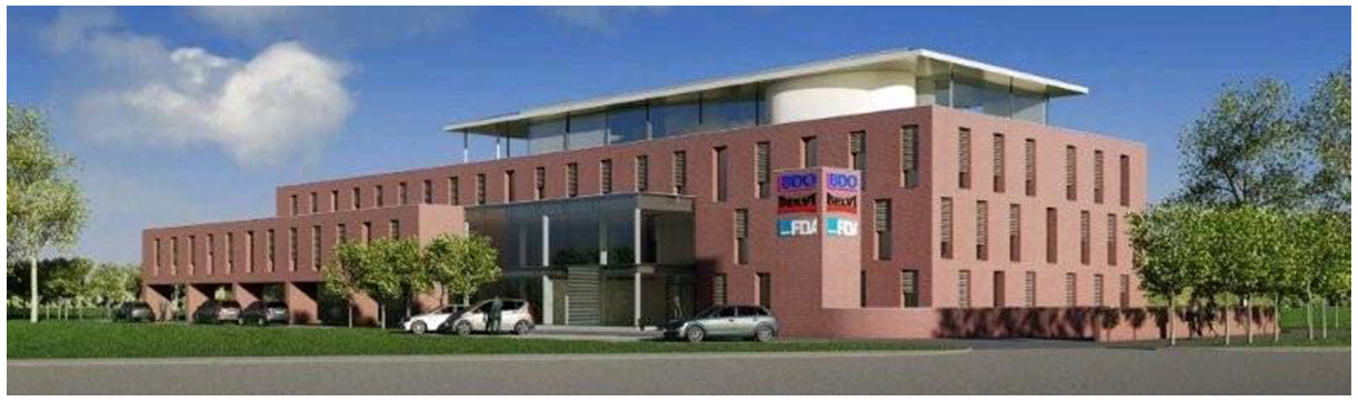
Fig. 9.10 Hollandsch Huys building (Hasselt, Belgium)

The building and its systems are monitored by a large set of built-in sensors. Historical data of these measurements since 2007 are stored, allowing a detailed analysis of the technical performance. The main difficulty in interpretation of these data lies in the fact that the building has not been fully rented and occupied by the time this study started. In 2007, about 75 percent of the second floor and the roof apartment was still vacant. From 2010, the second floor was used. The systems commissioning phase was not fully completed yet, resulting in control set points being tuned during the measurement period.

Since January 2013, the building is controlled intermittently during the heating season using model predictive control (MPC) instead of the traditional rule-based control (RBC). The MPC has been developed by the University of West Bohemia, Czech Republic (Jan Siroky) and the Czech Technical University in Prague, Czech Republic [Cig13] in collaboration with KU Leuven. The project (SMART GEOTHERM) aimed at analyzing the improvements obtained by the reduced-model-based MPC strategy, generalizing the results for different types of thermally activated building offices using geothermal energy and extracting a new RBC algorithm based on the MPC results. The analysis was done by a combination of simulations and experiments.

Fig. 9.11 shows the components of the thermally activated building.

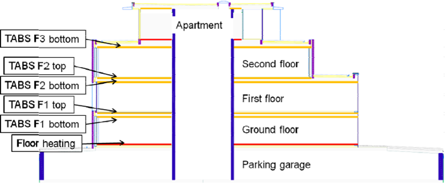
Fig. 9.11 Scheme of the thermally activated building components (floor heating: red, TABS: yellow)

The production unit in heating mode and the general layout of the simulation model are shown in Fig. 9.12 and Fig. 9.13, respectively.

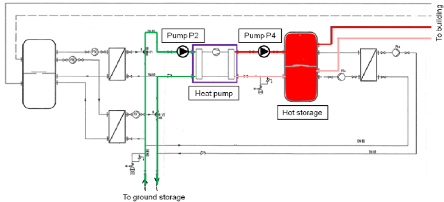
Fig. 9.12 Production unit in heating mode

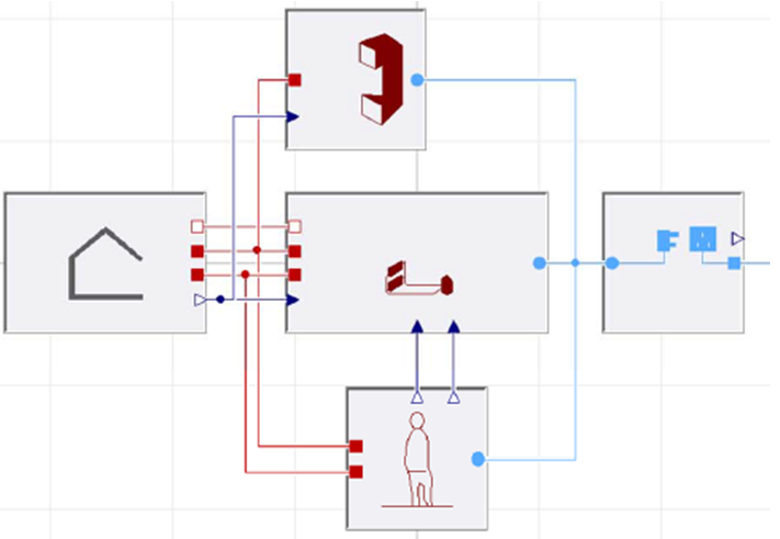
Fig. 9.13 General layout of the Modelica system simulation model, using the IDEAS-library. Left: building structure. Top: air handling unit. Center: heating/cooling production system. Bottom: internal gains due to occupancy. Right: electrical grid.

The building was simulated using the IDEAS-library developed by KU Leuven. The whole energy system was modeled in Modelica and simulated with Dymola.

9.2.5. Modeling for the Design of an Energy and Water Efficient Hotel

The case study deals with the HVAC, non-portable water and domestic hot water system of the newly constructed Grand Beach Hotel at Surfside, Florida, USA [MHB+15] (see Fig. 9.14).

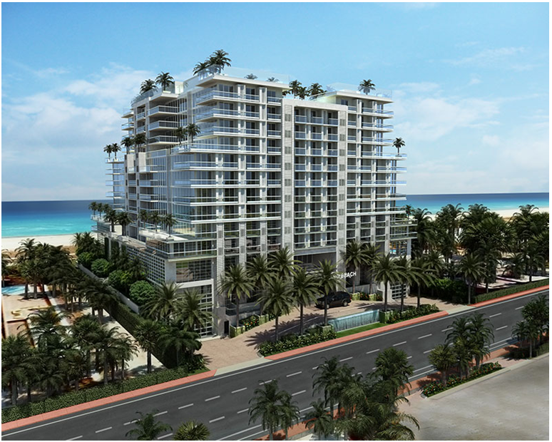
Fig. 9.14 Grand Beach Hotel at Surfside, Florida

To achieve the efficiency in energy and water, the HVAC, non-portable water and domestic systems are highly coupled. The collected rain water is used for non-portable water usage, such as flushing the toilet, and used as makeup water for the cooling tower. When condition allows, the domestic water will be pre-heated using the waste heat from the heat pump, and it will be used to reduce the cooling energy that is to be provided by the chilled water.

The simulation analysis was used for the system design and optimization. It helped the engineers decide the potential energy saving, balance the water pressure in the pipe system, and evaluate the control sequence.

Fig. 9.15 and Fig. 9.16 show the schematic HVAC and domestic water system and the corresponding Modelica models.

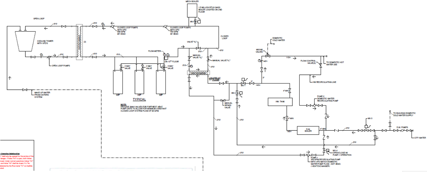
Fig. 9.15 Schematic of the HVAC and domestic water system

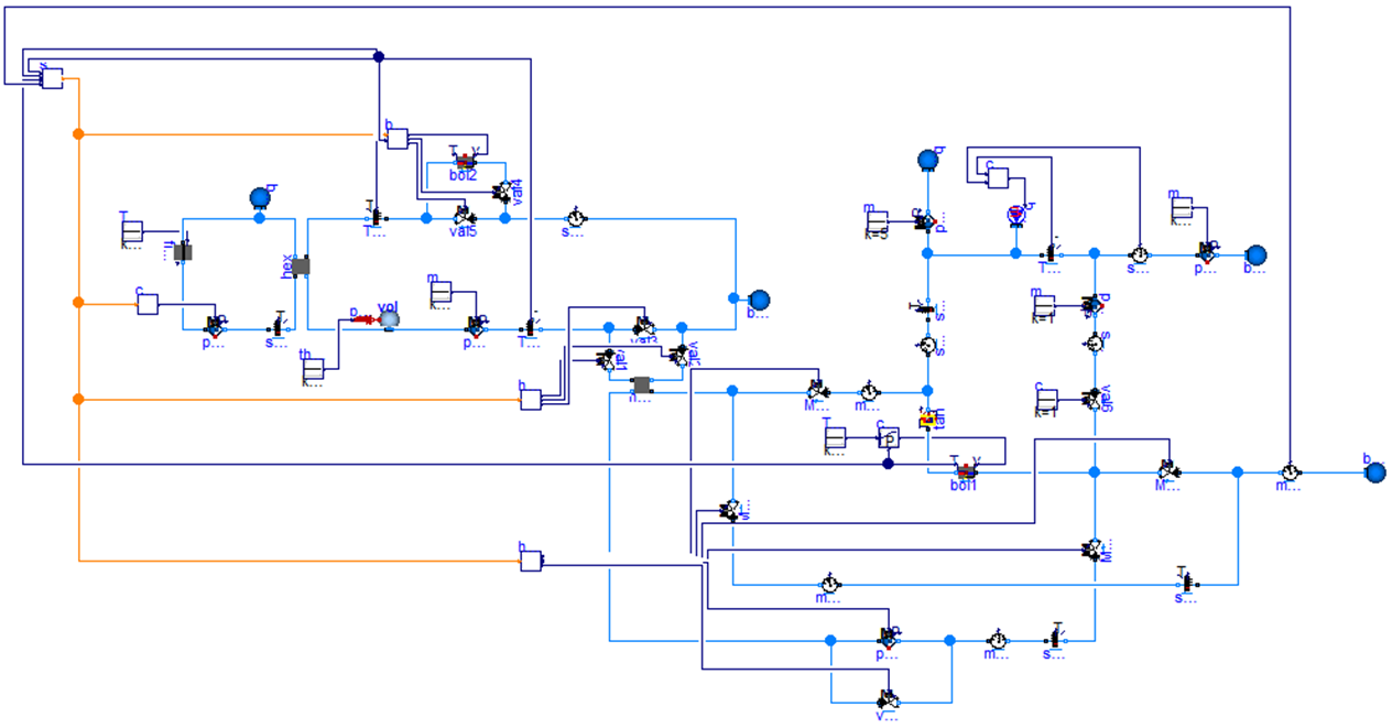
Fig. 9.16 Modelica system model of the same system

The system models for the simulation analysis were configured with the component models of the LBNL’s Buildings library [WZNP14]. The whole energy and hydraulic system was modeled in Modelica and simulated with Dymola.

9.2.6. Design of an Innovative Two-Pipe Chilled Beam System for Simultaneous Heating and Cooling of Office Buildings

This case study aims to design and evaluate energy performance of an innovative two-pipe system in active chilled beam application. The system enables simultaneous heating and cooling of office buildings by transferring energy between zones, using one hydronic circuit only. The system is designed to have the same inlet water temperature on the entire circuit. This temperature is controlled between \(20^\circ \mathrm{C}\) to \(23^\circ \mathrm{C}\), depending on the room air temperatures. Outlet hot and cold water is mixed together and as a result the system only needs to cool or heat the water to reach the inlet temperature again. By only having to cool or heat the water, no energy is wasted by doing both at the same time.

The possibility to design such a system was explored through a preliminary simulation-based research at the Danish Building Research Institute, in collaboration with Lindab A/S [ANHB13]. The system was modeled with BSim, a Danish building energy simulation tool, and integrated into a typical office building model. Standard internal gains for offices were set and thermal properties for the building envelope elements were selected according to Danish regulations. The building is located in Copenhagen (Denmark) and the correspondent weather file was used for the simulation. Results showed that the two-pipe configuration uses 3 percent less energy than a conventional four-pipe system.

However, BSim does not offer all the necessary features for a detailed design of the two-pipe system and some assumptions in the model were made. In order to be able to represent and control each single component of the system Modelica was chosen for more detailed studies.

Fig. 9.17 illustrates the principle of the two-pipe active chilled beam system. In this particular example, the inlet water temperature in the circuit is \(22^\circ \mathrm{C}\). The room located on the north facade needs heating and the outlet water temperature is \(20^\circ \mathrm{C}\). Conversely, the space located on the south facade needs cooling and the outlet water temperature is \(23^\circ \mathrm{C}\). As a result, the outlet water temperature in the circuit was \(21.5^\circ \mathrm{C}\). The system only needs to provide energy to reach \(22^\circ \mathrm{C}\). Fig. 9.18 shows the system model in Modelica used for the preliminary analysis.

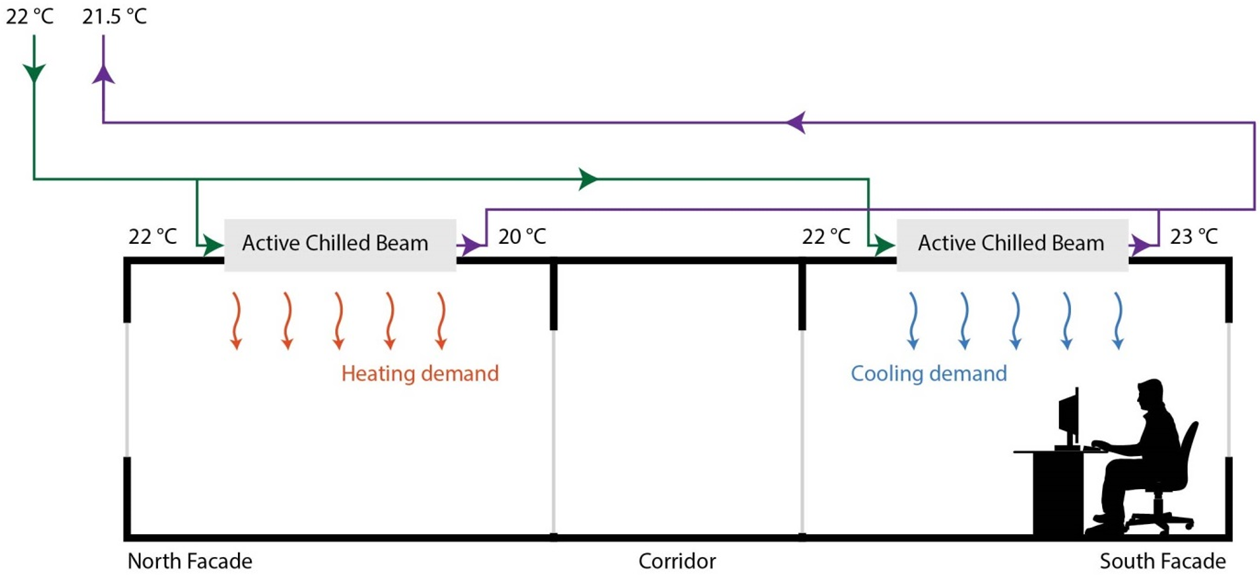
Fig. 9.17 Two-pipe active chilled beam system for simultaneous heating and cooling

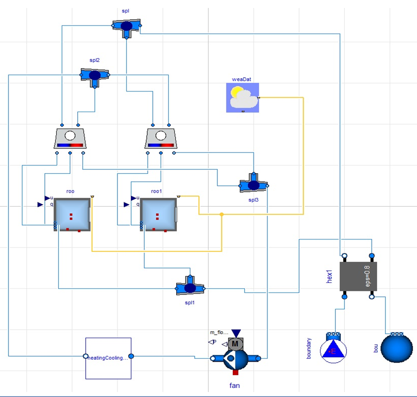
Fig. 9.18 Modelica model of the building system

After the preliminary study, a more detailed study was conducted, using a typical office building model. Simulations were run for two construction sets of the building envelope and two conditions related to inter-zone air flows. To calculate energy savings, a conventional four-pipe system was modelled and used for comparison. The conventional system presented two separated water loops for heating and cooling with supply temperatures of \(45^\circ \mathrm{C}\) and \(14^\circ \mathrm{C}\), respectively. Simulation results showed that the two-pipe system was able to use less energy than the four-pipe system thanks to three effects: useful heat transfer from warm to cold zones, higher free cooling potential and higher efficiency of the heat pump. In particular, the two-pipe system used approximately between 12% and 18% less total annual primary energy than the four-pipe system, depending on the simulation case considered [MWA+17].

The Buildings library from LBNL ([WZNP14]) was used for the system modeling, the energy analsysis and the controls design.

9.2.7. Integrated Optimal Design and Control of Office Buildings Using Renewable Energy Sources

This case study was performed in the PhD project “Integrated optimal design and control of office buildings using renewable energy sources” at the KU Leuven. The aim of this PhD project was to find a methodology for integrating optimal control and design of office buildings (compare with Fig. 9.19).

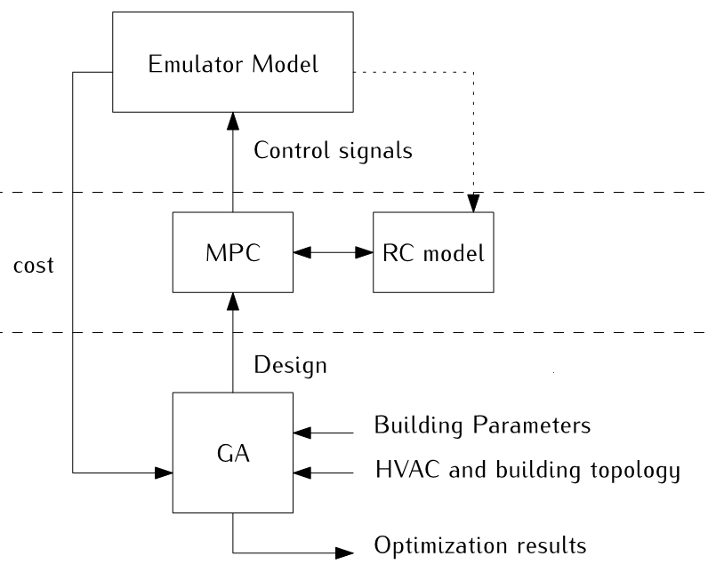
Fig. 9.19 General outline of the case

Usually, optimal control and design are solved as two independent problems. Optimal control is performed on a fixed design and optimal design is performed by assuming a simplified control sequence. However, technologies such as Concrete Core Activation (CCA) typically operate in a transient regime due to their large time constants. Furthermore the added value of renewable energy sources is difficult to assess without considering the entire system. This PhD project aimed to assess the potential of optimal control and optimal design using an integrated approach and dynamic simulations. This research proposed a methodology that optimally exploits this potential in practice so that the total costs (investment and running costs) are minimized. Modelica was used to create a parameterized emulator model of the building that needs to be optimized. A Model Predictive Controller (MPC) performed the optimal control of the building’s HVAC-system. A controller model (RC model) was used to limit the computational effort. The performance of this controller was evaluated using the Modelica emulator model. This control optimization was nested in a stochastic optimization that optimizes the design of the building with respect to building parameters, different HVAC-components, etc.

The IDEAS library [BDCVR+12] and the Buildings library [WZNP14] was used for this research in combination with Dymola.

9.2.8. Development of a Virtual Computational Test-Bed for Building Integrated Renewable Energy Solutions

In this case study, a virtual computational test-bed for building integrated renewable energy solutions was developed using Modelica. This test-bed helps assessing the full scale performance potential of existing products based on pilot scale testing results from the Eindhoven University of Technology (TU/e) campus and simulations which are calibrated using the pilot scale testing measurements. The pilot scale testing facility is a cooperation known as SolarBEAT (http://www.seac.cc/projects/solar-beat) which has been established between the TU/e and the Solar Energy Application Centre (SEAC), an independent research organization. This facility is being constructed on the roof of the Vertigo building, home of the Department of the Built Environment at TU/e. It consists of dummy buildings with building-integrated photovoltaic/thermal (BIPVT) solar collectors.

The end product of this work will be a complete building system simulating photovoltaic modules, solar thermal collectors, occupancy, ventilation, infiltration, heating system, domestic hot water demand and heat storage, as shown in Fig. 9.20. The virtual computational test-bed helps assessing the performance of different technologies. Those technologies will consist of BIPVT systems from different companies which are interested in testing their products and assessing their performance.

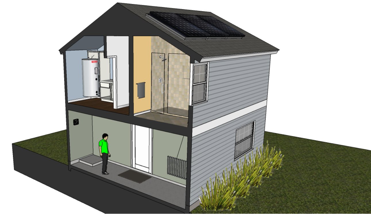
Fig. 9.20 Full home system schematic

The building is a single family house for 4 occupants. It is assumed that the house has 10 thermal zones: 3 zones at the ground floor including the kitchen, living room and the entrance, 5 zones in the second floor including 3 bedrooms and the second floor/attic which is divided into 2 rooms. The different zones are connected to each other thermally through the common walls and through the doors which can be controlled to be open or closed. However, the air connection between the different floors was not modeled.

The Modelica model consists of three major parts: the PV model, the solar thermal model and the house model. The house model was used to model the heating demand of the home. The first two models were used to model the generation of renewable energy for the given location of interest. Using the combined simulation, it was possible to analyze the dynamic interaction between the renewable generation systems and the energy demand of the home. The house is heated using typical radiators which are connected to the water heating system.

A complete heating system was modeled in this case study. The schematic in Fig. 9.21 illustrates a more detailed depiction of the solar thermal, space heating and domestic water heating system.

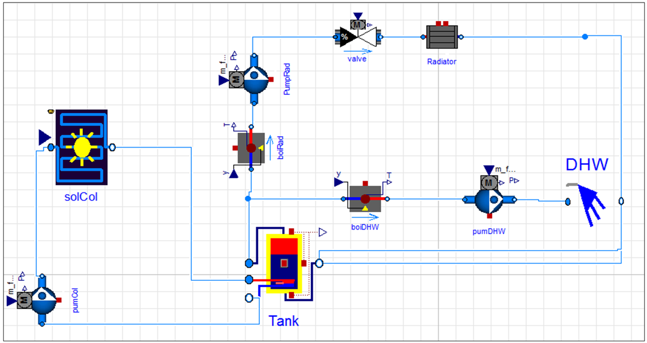
Fig. 9.21 Heating system schematic

This system contains a heat storage tank connected by a heat exchanger to an array of solar collectors. This tank is also connected to a boiler which heats the water to a specific temperature required by the heating system. The heating is provided by radiators in each of the thermal zones. Each of the radiators is controlled by a valve according to the set-point temperature. A pump in the collector circuit and another pump in the heating circuit ensure hot water circulation. Moreover, the domestic hot water circuit contains another boiler to ensure sufficient hot water temperature, and it contains a pump for the water circulation. All the components are controlled depending on the required temperature for the day, night and the outside temperature.

The electrical model should consist of an electrical network, representing the dwellings distribution system to which the PV and all power consuming equipment are connected. However, modeling different components inside the house and their energy consumption is a complicated task which requires the availability a well determined usage and occupancy profile. In the case of this work, the decision was made to represent the electrical demand using average measured data varying throughout the year.

The electrical power demand can vary according to the user behavior, the number of occupants and the resolution of the data available. For instance, a set of electric power demand data with a resolution of 5 minutes is more accurate than one with a resolution of 15 minutes. The 15 minutes data has flatter peaks of power demand due to its temporal averaging. Therefore, the higher the resolution, the more representative is the data [SHK14]. That being said, it is difficult to get access to detailed specific data from power companies due to privacy issues. The most complete data available for this application is an average consumption data for one house with a resolution of 15 minutes. The electrical network contains also a resistor representing losses and a voltage source to set the operating voltage as shown in Fig. 9.22.

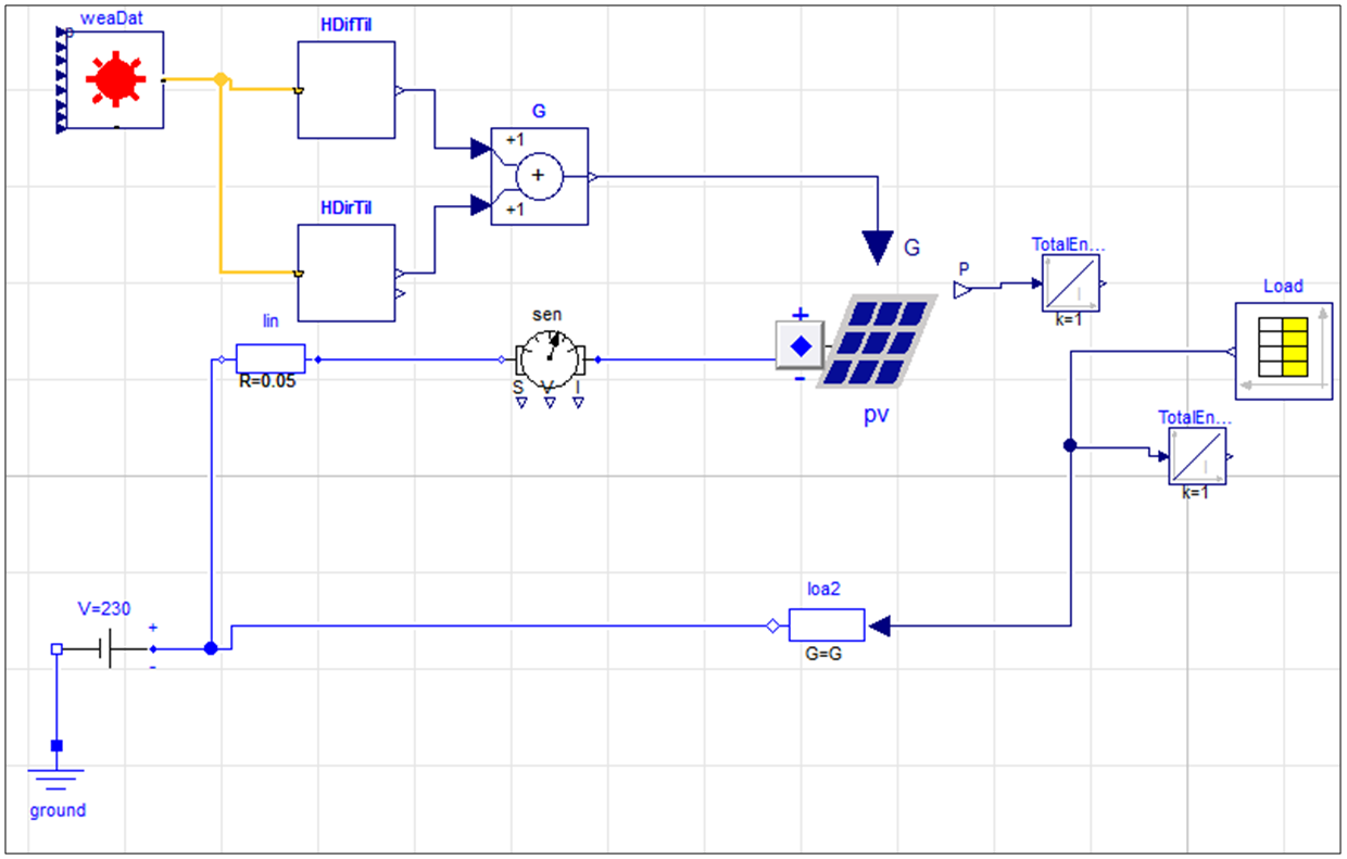
Fig. 9.22 Electric model containing the weather data, PV and the load profile

Fig. 9.23 represents the implementation of the model in Modelica. The block on the left contains the BIPVT and the heating system, while the block on the right represents the single family Dutch house. The top block is the weather data input.

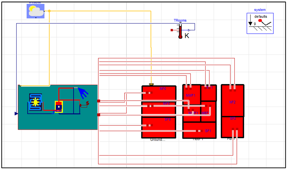
Fig. 9.23 Model implementation in Modelica

The system models for the simulation analysis were configured with the component models of the Buildings library from LBNL [WZNP14]. The whole energy system was modeled in Modelica and simulated with Dymola.

9.2.9. Influence of German Energy Saving Ordinances on Heat Demand of a Residential Building

This case study investigated the influence of different German energy saving ordinances on the heat demand of a residential building. In the past, German government had issued several energy saving ordinances, which define limits for the properties of building envelopes in order to reduce heat demands in new building construction. As these properties define the minimum requirement for all buildings built in a certain time period, they can help estimating a building’s properties given only its year of construction. Therefore, reference simulations of buildings with these standard properties can serve as benchmarks for a large share of Germany’s building stock and as the foundation for further investigations of the system or its parts.

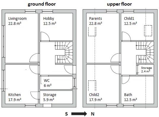
Fig. 9.24 Floor plan for the reference building

As a reference building for this case study, a one family dwelling with an area of 150 m²over two floors (see Fig. 9.24) was used. In order to only quantify the influence of the building envelope, each room is equipped with an ideal heater. For the location of this reference building, central Germany with weather input from the German test reference year region 12 was selected. The same building setup and weather input was used for building instances with envelope properties of energy saving ordinances from 1984, 1995, 2002, and 2009. Because this case study shall serve as a foundation for further studies, it was included as a demonstration example in the Modelica library AixLib [BM10][FCL+15]. Further details can be found in [CSM14].

The Modelica system model was built in a modular way, starting with wall elements including windows and doors. Several wall elements were grouped together to form a room model. The room models were connected to model a single floor. The floors can be connected to the outside environment and to heating system models to form a model of the entire building. In order to test the influence of different building envelope properties, upper-level parameters specify the wall constructions according to a chosen energy saving ordinance. Further parameters can be used to specify a light, medium or heavy building construction and air exchange rates. Thus, there is little manual effort needed to compare different building setups in a certain context. Through the modularity of the modeling approach, the building model could also be connected to a more elaborate heating system model with a prototype controller to test the control performance subject to different building properties. This allows engineers to quickly test their developments with a variety of typical German building setups.

The Modelica model of this building setup is shown in Fig. 9.25. The whole energy system was modeled in Modelica and simulated with Dymola.

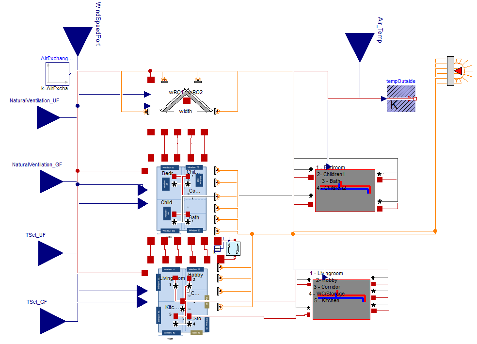
Fig. 9.25 This case study is an illustrative example of the library AixLib. It uses components from AixLib’s Building package as well as basic models from the Modelica Standard Library

9.2.10. Comparative Analysis of all Case Studies

A comparison of all nine case studies regarding the used Modelica libraries, the type of the component models and the used Modelica tools provides following information:

Used Modelica libraries: Different Modelica libraries were used for the case studies, 3 times the Buildings library from LBNL, 3 times the IDEAS library from KU Leuven, once the BuildingSystems library from UdK Berlin. Further specialized Modelica models were used by the Fraunhofer institute ISE, which are not part of the publicly available Modelica libraries.

Used Modelica component models: A wide range of energy plant models and thermal building models were used in the case studies:

• Auxiliary models:

  • Controllers (Two point-controller, PI controller)
  • Data reader & interpolation (e.g. weather data, user behavior)
  • Radiation calculation on tilted surfaces

• Energy transformation models:

  • PV module and generator with maximum power point tracking
  • Solar thermal collector
  • Electric driven heat pump and chiller
  • Borehole heat exchanger for ground coupled heat pumps
  • Cooling tower
  • Boiler (e.g. condensing gas, wood pellet)
  • HVAC: adiabatic cooling, mechanical cooling

• Energy storages Models:

  • Electric battery
  • Thermal water storage (cold water, hot water)
  • Bore-field

• Energy transport models:

  • Thermo-hydraulic components: pipe, branch, two-way and three way valves, constant and variable speed pump
  • HVAC components: ducts, ventilators, heat recovery components
  • Heat emission systems such as radiators and floor heating
  • Heat exchangers
  • Heat emission components: TABS, radiators, active beams

• Building models:

  • Simplified thermal building model (one zone)
  • Detailed building model (multiple zones)

Used Simulation Tools: In all of the case studies, Dymola was used as the Modelica simulation tool. (When the case studies were conducted, Dymola was the only tool that could simulate all used models. However, as of Spring 2017, JModelica fully supports the Annex 60 library and the Buildings library.) In two cases, EnergyPlus was used in addition by co-simulation, based on BCVTB (https://simulationresearch.lbl.gov/bcvtb). In one case study GAMS (http://www.gams.com) was used for an operational model.

In two of the case studies, optimization analysis with GenOpt(https://simulationresearch.lbl.gov/GO/) were done. One case study used a Python-framework for the realization of a model-based predictive control (MPC). One case study used the MATLAB toolbox YALMIP (http://users.isy.liu.se/johanl/yalmip/pmwiki.php?n=Main.HomePage) for optimization.

9.2.11. Reasons for the Use of Modelica

The reasons for the use of Modelica as stated by the case study participants can be clustered into the following groups:

Flexible and extensible object-oriented modeling approach: The object-oriented modeling approach leads to a high working efficiency and supports a transparent and clear understanding of component and system models. Hereby, an easy manipulation, re-use and/or adaption of existing component models is possible and missing component models can be easily implemented. The graphical and hierarchical modeling approach enables a well-structured and clear modeling process and supports system models with different levels of detail in the sub-models (e.g. a detailed plant model in combination with a simplified thermal building model). The combined use of existing large Modelica libraries enables new system models, which are normally not present in existing simulation tools.

Acausal equation-based modeling approach: The equation based approach leads to an easy understanding of the physical modeling of existing models and newly implemented models. It also gives a good physical insight in the problem and the components. The result is a clear understanding of the underlying physical-technical equation system at the component and system level. Especially the non-causal approach of Modelica supports necessary features in energy plant simulation domain such as the bi-directional mass flow within thermo-hydraulic networks.

Multi-domain approach: The multi-physical modeling approach of Modelica including the domain specific common interface definitions supports the integration of domain specific sub-models into a common system model (e.g. building physics, hydraulics and electrical grids).

Numerical reasons: The automatically translation of the textual Modelica model into a running simulation model with time integration allows the modeler a clear separation between the physical-technical model itself and its numerical solution.

External interfaces to Modelica: Modelica-models can be easily coupled with external optimization software (e.g. GenOpt and GAMS). The scripting language Python can control Modelica simulation tools and can serve for pre-and post-processing steps. Co-simulations of Modelica with other simulation tools are possible, e.g. with BCVTB and/or FMI. One typical example is the co-simulation of a HVAC system, modeled in Modelica and a multi-zone building model in EnergyPlus.

Collaborative development: The modular approach of Modelica supports common software development within single teams, and also within a broader distributed model development such as done for the Annex 60 library that was developed in Activity 1.1 and is used in major Modelica libraries for building energy applications.

9.2.12. Drawbacks of Using Modelica

The authors of the case studies have stated the following most important drawbacks by using the Modelica language, Modelica libraries, or Modelica tools in the context of building energy simulation:

Long simulation times for detailed whole building simulation: Whole building simulations are often slower than with dedicated building energy simulation programs, in particular if detailed HVAC models are combined with multi-zone building envelop models. This has several reasons: First, Modelica models often include more detail than for example an EnergyPlus or TRNSYS simulation. Typical examples include modeling of realistic control sequences and pressure-driven mass flow distribution in pipe and duct networks. Second, numerical solvers in the tools use the same time step for all equations. However, for building envelope heat conduction, much larger time steps could be used than what is required for control loops. Here, the use of multi-rate solvers with error control is promising. Third, if an event is triggered by a model, then the whole time integration is stopped, and the integration is restarted, typically with a low order integration method. However, many events could be treated in a subsystem, in particular if they affect other parts of the model through integrators, as integrators smoothen discontinuities. Fourth, Modelica translators typically convert the models to a dense system of equations rather than preserving the sparsity, which then could be exploited using sparse solvers. Fifth, ordinary differential equation solvers for stiff equations that scale cubic in the number of state variables are often used. This can lead to large computing time if the building envelope model, with many slow evolving states, and the HVAC model, with few but fast evolving states, are coupled. However, research and development is ongoing on all of these issues, and they are not an inherent problem of the Modelica language which for simulation is converted to efficient C-code, as described in Section 5.3.4. Rather, it is a problem of the solvers that are currently in use and need to be improved as users simulate larger Modelica models than they did in the past. At the time of this writing, various research in such model translations and numerical methods that allow faster simulation is ongoing, see for example [MBKC13][FBC+14][Cas15][BBCK15][BRC16][CR16][OE17][BCB17][JHB17]. As Modelica separates declarative model formulations from solution methods, these methods can be made available in simulation environments with little to no changes to the underlying model libraries.

Reliance on one commercial Modelica tool: During the research phase of this project (2013 to 2016), only Dymola supported the entire Modelica language specification. Hence, complex Modelica system model run only partly with other commercial or open Source Modelica tools. Since Spring 2017, the situation is improving as the open source Modelica tool JModelica works with the Annex 60 library and the Buildings libary, and other tool providers stated that they are working on increasing the support of models that are used for building energy simulation.

Connector types were not standardized: At the start of the Annex, some Modelica libraries used connectors and function that compute enthalpy as a function of temperature that were different from the ones standardized in the Modelica Standard Library. This made combining existing models difficult as adapters had to be implemented. In the meantime, the Annex60, AixLib, BuildingSystems, Buildings and IDEAS libraries all use the same adapters and media functions, making their models compatible.

Fewer validated models than established building simulation programs: Modelica offers fewer models than for example EnergyPlus or TRNSYS, and since the libraries are new compared to these established tools, the range of validated models is smaller. However, Modelica libraries are more transparent in comparison to EnergPlus, in particular regarding how components and systems are controlled. Also increasing the scope of models and their level of validation was a key motivation for the development of the Annex 60 library as a common base for different Modelica libraries. See also Section 5.4.5 for the quality control in the Annex 60 library.

9.3. Model Analysis

Outgoing from the described case studies, an analysis about the used Modelica models of the four libraries for building energy and plant simulation AIXLib, BuildingSystems, Buildings, and IDEAS was performed. Because the quantity of all of the used Modelica component models was large, only models used in one or several of the case studies were considered in the analysis.

In the second step, a comparison between the spectrum of the used models and the present models of the Annex 60 library (version during Fall 2014) were conducted. In this manner, commonly used models were identified. This served as a basis to prioritize which new component models to add to the Annex 60 library. This fits with the idea of the Annex 60 project of providing a core Modelica library, while allowing individual libraries to differ in the specialized models that they provide.

The following ranking was obtained by the statistics of how often a Modelica model was used in all of the case studies and was not present during Fall 2014 in the Annex 60 library:

1. Compression chiller/heat pump; Thermal zone models or building models: 6 x
2. Radiation calculation for tilted surfaces: 5 x
3. Thermal water storage (hot water/cold water): 4 x
4. Data reader / interpolator: 3 x
5. Borehole heat exchanger; Cooling ceiling / radiant slab; Photovoltaic model: 2 x
6. Solar thermal collector model; thermally activated building systems; electric battery model; Cooling tower: 1 x

Starting from this case, the following five most used models should be integrated in the future versions of the Annex 60 library:

A simplified thermal building model: In the majority of case studies, the building energy and plant simulations were coupled, with the focus of the analysis being on the plant. The building model delivered the dynamically calculated heating and cooling demand, typically in yearly simulations. Hence, a simplified thermal building model is needed.

A thermal water storage model: Many thermal energy concepts used a thermal storage tank to store hot or cold water. They are integrated in hydraulic concepts in different manners (e.g. internal/external heat exchangers) and also often the thermal stratification is important (e.g. for solar thermal systems). Hence, a thermal horizontal 1D-discritized tank model with flexible inputs and outputs should be part of the Annex 60 library.

A compression chiller/heat pump model: Many energy concepts are based on (reversible) heat pumps and/or compression chillers. Hence, a simplified model should be included in the library, which uses characteristic curves for fast system simulation analysis.

A solar radiation calculation model: One basic feature consists in the transformation of horizontal solar radiation as obtained from the weather data into the incident irradiation on tilted surfaces (e.g. building envelope, solar thermal collectors, photovoltaic modules).

A data reader model: All building and plant system models have to read discrete, typically hourly, weather data, which have to be transformed into continuous boundary conditions for the building and its HVAC system. Hence, a data reader model which supports different types of interpolation should be part of the Annex 60 library.

9.4. OD/OC Method Analysis

Methods for optimal design and optimal control were used in following of the case studies:

• Multi-criteria optimization of PV-cooling systems for residential buildings (Section 9.4.1, TU Berlin, UdK Berlin, Germany), and
• Model predictive control framework (Section 9.4.2, KU Leuven, Belgium).

9.4.1. Multi-Criteria Optimization of PV-Cooling Systems for Residential Buildings

Optimization problem: A residential building in a hot climate region with space for two families (net floor area of \(278 \, \mathrm{m^2}\)) is air-conditioned by a solar PV cooling system. The optimization problem was analyzed for two different climate locations in the MENA region: The city Hashtgerd in Iran and the city El Gouna in Egypt [NGHN13]. The maximum air temperatures in Hashtgerd and El Gouna are nearly the same (41°C), but the mean temperature during the summer period in El Gouna (30.4°C) is much higher than in Hashtgerd (26.0°C). The yearly horizontal global solar radiation is about \(1,800 \, \mathrm{kWh/(m^2 \, a)}\) in Hashtgerd and \(2,400 \, \mathrm{kWh/(m^2 \, a)}\) in El Gouna.

The mean U-value of the thermal envelope of the considered building was \(0.593 \, \mathrm{W/(m^2 \, K)}\) for walls, windows and roof, and \(0.350 \, \mathrm{W/(m^2 K)}\) for the floor. The potential surface for PV modules on the roof was about \(135 \, \mathrm{m^2}\).

The study aims to solve a multi-criteria optimization of the PV cooling system. Furthermore, the PV cooling system has to supply 100 percent of the cooling demand by solar energy without any use of additional electricity from the grid.

For this purpose a cost-function with three different design criteria was defined:

1. Over temperature: The first criteria was to avoid overheating for an optimal thermal comfort. If the indoor air temperature exceeds the set temperature of 26°C, then the difference TAir-TSet (over temperature) was integrated over time.
2. Investment costs: The second criteria was the minimization of the investment costs. The following assumptions to the specific investment costs were made: (PV generator: 0.7 Euro/\(W_{peak}\); Battery: 600 Euro/kWh; Compression chiller: \(0.4 \mathrm{Euro}/W_{el}\); Cold water storage: costs in \(Euro = 1649.81 \, V^{-0.464}\) where \(V\) is the storage volume.
3. Durability of the components: The third criteria was the reduction of switching on/off events of the compression chiller.

These three criteria were weighted with the factors \(f_1=1\), \(f_2=1\) and \(f_3=2\). Electricity costs were not considered, because the PV cooling system works grid-independently.

These chosen optimization parameters and the possible parameter spans for the optimization algorithm were as follows:

1. Number of PV modules: 1 to 83,
2. Capacity of the electric battery: 1 to 80 kWh,
3. Nominal power of the compression chiller: 0.1 to 5.0 kW and
4. Volume of the cold water storage: \(0.1 \, \mathrm{m^3}\) to \(10.0 \, \mathrm{m^3}\).

Used Modelica system model for optimization: The PV cooling system was modeled in Modelica by the use of the BuildingSystems library. It consists of the following seven main sub-models which are also shown in Fig. 9.26:

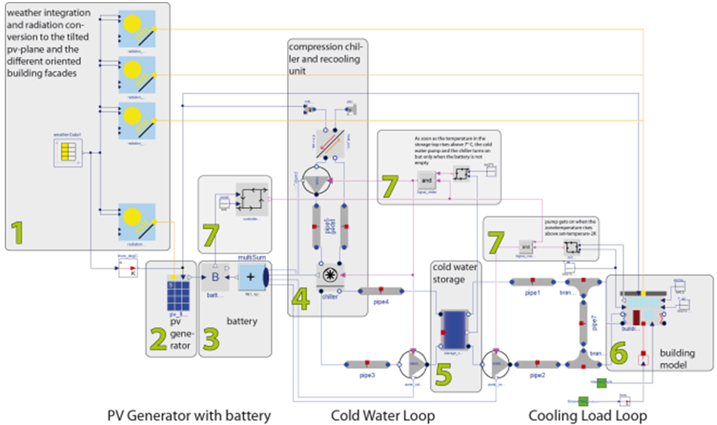
Fig. 9.26 Modelica system model of the PV cooling system and its sub-models

1. A weather data reader and its conversion to different surfaces (PV surfaces and building facades),
2. a PV generator system model,
3. an electrical battery model,
4. a model of a compression chiller with its recooling unit,
5. a cold water storage model,
6. a simplified thermal building model,
7. controller models.

Several controllers were implemented within this system model. The first controller manages the cooling load pump. This pump switches on if the room air temperature reaches the set temperature with an offset of 2 K. The second controller measures the water temperature in the top of the cold water storage. If the temperature rises above 7°C, the compression chiller, the re-cooling pump and the cold water loop pump turns on, but only if the battery load state is not lower than 20% (discharge protection).

Used method and tools for optimization: The GenOpt framework (http://simulationresearch.lbl.gov/GO/) was used for the parameter optimization problem. GenOpt varies predefined parameter sets within the admissible parameter bounds, dependent on the selected optimization algorithm. It then starts the Dymola simulation for one year, and the simulation model writes the cost function value to a file that will be read by GenOpt. Dependent on the progress of the optimization, Genopt varies the parameter set again for the next simulation run until a convergence criterion is satisfied. The GPSHookeJeeves algorithm was used for the optimization problem.

Results of the optimization: GenOpt was started at both climate locations with the same parameter set:

• Number of PV modules: 70,
• capacity of the electric battery: 40 kWh,
• nominal power of the chiller: 1.0 kW,
• volume of the cold water storage: \(5.0 \, \mathrm{m^3}\).

After 120 simulations, the cost-function for both locations has converged, as shown in Fig. 9.27.

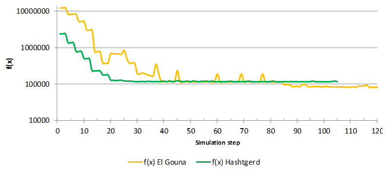
Fig. 9.27 Final cost-function value and its composition for the locations El Gouna and Hashtgerd

The cooling load in Hashtgerd leads to higher peak values. However, the yearly cooling energy in El Gouna is higher than in Hashtgerd, because of its higher mean temperature. The maximum temperature during the summer is nearly the same at both locations.

For these reasons, the optimization algorithm has found for Hashtgerd the same number of PV modules (83). This is maximum value of possible modules on the roof area. The location El Gouna with a higher mean temperature and cooling demand needs greater storage capacities for cooling energy. The daily and yearly timeline of the solar irradiation is more balanced in comparison to Hastgerd. Consequently, the optimization algorithm calculated for El Gouna a larger and cheaper cold water storage \((6.1 \, \mathrm{m^3}\) instead of \(5.5 \, \mathrm{m^3}\)) and reduced the capacity of the electric battery (40 kWh instead of 55 kWh) in comparison to Hashtgerd.

Fig. 9.28 shows the detailed investment costs for both locations. The main costs are from the battery and the PV generator. The costs of the cold water storage and the chiller are less significant.

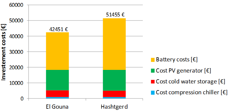
Fig. 9.28 Investment costs in Euro for both locations

The PV cooling system causes in Hashtgerd a higher overheating time (16.9 hours) as in El Gouna (10.8 hours) caused by the higher cooling load peaks. Because of the higher alternating external temperature, the compression chiller switches on more often in Hashtgerd (355 times) than in El Gouna (270 times).

9.4.2. Model Predictive Control Framework

Model Predictive Control (MPC) is a control strategy that can be applied to building applications. The idea of MPC is to create an optimization problem that optimizes the control variables (valve positions, heat flow rates) such that the operation point with the lowest cost is obtained that still satisfies comfort constraints and other constraints that may be imposed. An MPC problem estimates future energy use under consideration of weather and occupancy forecasts. Hence, it anticipates future solar gains, thereby possibly reducing the heating power or pre-cooling the building at night when cooling is typically cheaper. Comfort constraints are typically formulated based on zone operative temperatures. Depending on the complexity of the model that is used to estimate energy use, the optimization problem may be categorized into different problem classes such as a Linear Programming (LP), Quadratic Programming (QP), Nonlinear Programming (NLP) etc. Efficient specialized optimization solvers exist depending on the problem class. LP’s can for instance be solved very quickly. Each of these solvers however requires that the equalities, inequalities, cost function and input data defining the problem are provided to the solver in a certain format. Obtaining these equations and data requires knowledge of specialists, especially for large problems.

Classical building simulation tools typically do not allow the automated extraction of these model equations or input data. The model equations of individual component models may be publicly available, but using these directly would again require the equations to be recombined manually when individual component models are coupled. Modelica offers some interesting advantages in this respect, which may greatly simplify extracting models for use in MPC. First, open source libraries exist where the users has control over the type of equations, meaning that component models may be simplified to match a certain problem class. For instance, a library of linear building component models may be constructed if the user wants to obtain a LP controller model. Second, Modelica simulation environments allow any variable to be stored in an output file, and therefore the required input data can be exported. Third, Modelica simulation environments typically allow to linearize a model and extract a linear state space formulation of the problem in the form

(1)\[\begin{split}\dot{x} &= A \, x + B \, u, \\ y &= C \, x + D \, u,\end{split}\]

where \(x\) are the problem states, \(\dot{x}\) is the time derivative of \(x\), \(u\) are model inputs and \(A, \, B, \, C, \, D\) are constant matrices. When linearizing a model, these matrices are computed. Fourth, specialized Modelica solvers such as JModelica and OpenModelica allow to directly optimize the model equations without needing to export them first. At the time of this writing, their solvers, however, conservatively assume that the problem is a non-linear programming (NLP) problem, which increases the computation time compared to using a solver for linear programming (LP) problem.

Using these properties of the Modelica language and their solvers, an automated way for creating and exporting linear controller models with matching input data may be set up. A first step would be to create a building model in Modelica using a library that contains only linear equations. Second, a state space model of the form (1) needs to be extracted. Third, an input data file needs to be generated that matches the inputs \(u\) of the state space model. Then, these data can be used by an efficient LP optimization algorithm to compute optimal control results. Note that an interesting feature of Modelica is that the optimization algorithm, which is not implemented in Modelica, may be compiled into C-code that may be called from Modelica. This way, an MPC controller may be embedded into a Modelica model, which removes the need for co-simulation techniques.

This approach was used at the KU Leuven to set up an automated Model Predictive Framework using the IDEAS library. In [PJH15] the linearization approach is outlined. In [JH16] the framework is explained and applied to an office building. In [PSJ16] the framework’s performance is compared to a grey box approach.

9.4.3. Optimal Control of Room-Level HVAC and Facade Control

This example demonstrates the use of collocation methods to solve a constrained nonlinear optimal control problem, and compares its computing performance to a gradient free optimization method. The example demonstrates the benefits obtained through the problem manipulation that the Modelica language allows due to its declarative nature.

9.4.3.1. Optimization Problem

The example minimizes sensible cooling, heating and fan energy demand for a thermal zone of a variable air volume flow (VAV) system by adjusting the time profiles of the supply air mass flow rate, the shading device control signal and the reheat power at the terminal box, subject to comfort constraints. Our application requirements are that the optimizations of individual zones are decoupled from each other, and that the central HVAC system can have its own control. For our example, the central HVAC system will supply air at \(18^\circ \mathrm C\) and at a relative humidity required for humidity control.

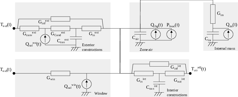
Fig. 9.29 Simplified model of a thermal zone.

Fig. 9.29 shows the simplified thermal model of the zone. Separate models exist for exterior constructions, partitions to adjacent zones and internal mass. These constructions are characterized by thermal capacitors and thermal conductance that account for heat conduction and convection. There is also a thermal conductor for infiltration.

The windows were modeled with a thermal conductance \(G_{win}\) and a power source \(Q_{sol}^{win}(t) = S_{rad}(t) \, A_{win} \, SHGC \, \chi(u_{win}(t))\), where \(S_{rad}(t)\) is the total solar radiation per unit area towards the window normal direction, \(A_{win}\) is the glass area, \(SHGC\) is the solar heat gain coefficient of the window, \(u_{win}(t) \in [0,1]\) is the position of the blind, and \(\chi \colon \Re \to \Re\) is a function that models the impact of the blinds on the fraction of solar radiation that enters the zone. The contribution due to solar radiation on the external constructions is \(Q_{sol}^{ext}(t) = S_{rad}(t) \, A_{ext} \, \alpha\), where \(A_{ext}\) is its area, and \(\alpha\) is the solar absorption coefficient of the exterior surface. The thermal conductance \(G_{im}\) models the heat transfer between the air and the internal mass. The power sources \(Q_{ihg}(t)\) and \(Q_{im}(t)\), respectively, model the internal heat gains that contribute to the zone air and internal mass. The internal heat gain is defined as \(Q_{ihg}(t) = P_{occ}(t) + P_{lights}(t)+ P_{plug}(t)\), where \(P_{occ}(t)\) is the internal heat gain due to occupancy, \(P_{lights}(t)\) is the internal heat gains due to lights, and \(P_{plug}(t)\) is the internal heat gains due to the plug loads. The power delivered by the HVAC system is \(P_{\mathit{hvac}}(t) = P_{hea}(t) + P_{sup}(t) + P_{fan}(t)\), where \(P_{hea}(t)\) is the power released by the reheating coil in the VAV box, \(P_{fan}(t)\) is the fan power, and \(P_{sup}(t)\) is the cooling power provided by the supply air from the central HVAC system through the VAV box.

The latter is \(P_{sup}(t) = \dot{m}_{air}(t) \, c_p \, (T_{sup}(t) - T_{air}(t))\), where \(\dot{m}_{air}(t)\) is the mass flow rate of air passing through the VAV box, \(c_p\) is the air specific heat capacity, \(T_{sup}(t)\) is the temperature of the supply air entering the VAV box and \(T_{air}(t)\) is the temperature of the air in the zone.footnote{Note that the computation of \(P_{sup}(t)\) is approximate to decouple the individual optimizations of multiple zones from each other. This was done to reduce the dimensionality of the optimization and to allow them to be solved in a distributed way.

The actual sensible cooling provided by a cooling coil in a system with economizer is \(\bar P_c(t) = \dot{m}_{air}(t) \, c_p \, (T_{sup}(t) - (T_{mix}(t) + \Delta T_{fan}(t) ))\), where \(T_{mix}(t)\) is the mixed air temperature after the economizer and \(\Delta T_{fan}(t)\) is the temperature raise over the fan. If \(y_{out}(t) \in [0, 1]\) is the outside air fraction, this becomes \(\bar P_c(t) = \dot{m}_{air}(t) \, c_p \, ( T_{sup}(t) - T_{air}(t) + y_{out}(t) \, (T_{air}(t) - T_{out}(t) ) - \Delta T_{fan}(t) )\). As \(y_{out}(t)\) and \(\Delta T_{fan}(t)\) (through the fan efficiency) depends on the mass flow rates and return air temperatures of other zones, these terms have been neglected in order to decouple the individual zone-level optimizations.} The power of the fan is \(P_{fan}(t) = P_{fan}^{nom}(\dot{m}_{air}(t)/\dot{m}_{air}^{nom})^3,\) where \(\dot{m}_{air}^{nom}\) is the nominal supply air mass flow rate, and \(P_{fan}^{nom}\) is the fan power required to supply \(\dot{m}_{air}^{nom}\) to the zone. Weather data for Sacramento, CA, have been used.

The described model was implemented in Modelica. The model can be described as an initial-value ordinary differential equation. Thus, it is a special case of the generalized DAE system, in which the algebraic constraints \(Y(\cdot, \cdot, \cdot, \cdot, \cdot)\) are absent. Therefore, the state variables, control functions and parameter are

\[\begin{split}x(t) &= [T_{air}(t), \, T_{im}(t), \, T_{con}^{int}(t), \, T_{con}^{ext}(t)], \\ u(t) &= [\dot{m}_{\mathit{air}}(t), \, u_{win}(t), \, P_{hea}(t)], \\ \Theta &= [T_{air}(t_0)].\end{split}\]

The energy consumption of the HVAC system is

\[E(t_f) = \int_{t_0}^{t_f} (-P_{sup}(t) \, \eta_{coo} + P_{hea}(t) \, \eta_{hea} + P_{fan}(t)) \, dt,\]

where \(\eta_{coo}\) and \(\eta_{hea}\) are coefficients that represents the efficiency of the HVAC system to provide cooling and heating. These typically include the coefficient of performance of chillers or heat pumps, or the efficiency of the furnace, as well as the effect of free-cooling by the economizer. The optimization variables are the time profiles for the control signals of the supply air mass flow rate \(\dot{m}_{\mathit{air}}(\cdot)\), the blind position \(u_{win}(\cdot)\), the reheat power \(P_{hea}(\cdot)\), as well as the initial zone temperature \(T_{air}(t_0)\). We modified the equation for \(E(t_f)\) to balance the weights of all its terms, obtaining

\[E_\gamma(t_f) = \int_{t_0}^{t_f} (-\gamma^1 P_{sup}(t) \eta_{coo} + \gamma^2 P_{hea}(t) \eta_{hea} + \gamma^3 P_{fan}(t)) \, dt,\]

where \(\gamma \in \Re^3\), with \(\gamma^i > 0\) for all \(i \in \{1, 2, 3\}\), are constants.

The optimal control problem is formulated as

\[\begin{split}\underset{u(\cdot) \in \, \mathcal{U} }{\text{minimize}} \qquad E_\gamma(t_f) + \int_{t_0}^{t_f} \kappa \, u_{win}(t)^2 \, dt,\\ \text{subject to} \qquad F(t, \, \dot{x}(t), \, x(t), \, u(t), \, y(t), \, \Theta) = 0,\\ F_0(\dot{x}(t_0), \, x(t_0), \, u(t_0), \, y(t_0), \, \Theta) = 0,\\ T_{air}^l(t) \leq T_{air}(t) \leq T_{air}^u(t),\\ 0 \leq u_{win}(t) \leq u_{win}^u(t),\\ \dot{m}_{air}^{l} \leq \dot{m}_{air}(t) \leq \dot{m}_{air}^{u},\\ P_{hea}(t) \geq 0,\\ T_{air}(t_0) = T_{air}(t_f),\end{split}\]

for all \(t \in [t_0, \, t_f]\), where \(\mathcal{U}\) is the set of admissible control functions \(u(\cdot)\), \(\kappa \in \Re^+\) is a constant, \(T_{air}^l(t)\) and \(T_{air}^u(t)\) are the lower and upper bounds of the comfort region of the air temperature, \(u_{win}^u(t)\) is the maximum admissible value for the control signal of the blind, and \(\dot{m}_{air}^l\) and \(\dot{m}_{air}^u\) are the minimum and maximum supply air mass flow rates for the zone.

The cost function includes an additional term that penalizes excessive control actions of the windows. For example it penalizes deploying the blinds at night. The equality constraint imposes that the temperature of the air at the start and at the end of the optimization period are the same.

9.4.3.2. Used Method and Tools for Optimization

The optimization problem was solved using JModelica [AGT09], using the collocation method described in Section 4.2.3 and solved the finite dimensional NLP problem with IPOPT version 3.11.9, and with the linear solver mumps.

For comparison of the computation time, the optimization problem was also solved using the Nelder-Mead algorithm, a derivative-free algorithm that is implemented in JModelica. For the solution with the collocation method, \(n_e = 48\) elements was used, each being \(30\) minutes long. For each element, three collocation points were used. The optimization ran for a summer day.

To assess the performances of the collocation-based method, it was compared with the simulation-based Nelder-Mead optimization algorithm. The Nelder-Mead algorithm can be applied to nonlinear optimization problems where derivatives are not available, as is the case with conventional building simulation programs. See [WW04] for a comparison among the Nelder-Mead and other derivative free methods. The optimization variables in the Nelder-Mead optimization problem are the initial temperature of the air in the zone, the control signal for the blinds, and the supply air mass flow rate. To reduce the size of the optimization problem, it was simplified for the Nelder-Mead optimization as follows: The heating power was set to \(P_{hea}(t) = 0\) for all \(t \in [t_0, \, t_f]\), and both the supply air mass flow rate \(\dot{m}_{\mathit{air}}(t)\) and the blind control signal \(u_{win}(t)\) was discretized using one-hour rather than \(30\) minutes intervals. The decision to choose no heating is appropriate for this hot day. Therefore, the optimization variables are

\[\begin{split}z &= [T_{air}(t_0), \, \dot{m}_{\mathit{hvac}}(t_0), \dot{m}_{\mathit{hvac}}(t_0 + \Delta t), \ldots , \dot{m}_{\mathit{hvac}}(t_0 + 24 \, \Delta t), \nonumber \\ & \qquad u_{win}(t_0), \, u_{win}(t_0 + \Delta t), \ldots , u_{win}(t_0 + 24 \, \Delta t)].\end{split}\]

Hence, the total number of variables to optimize is \(n_z = 51\). Let \(\tau = \{ t_0 + i \, \Delta t \}_{i=0}^{24}\). The cost function minimized by the Nelder-Mead algorithm is

\[\begin{split}f_{NM}(z) &= E_\gamma(t_f) + \mu_j \left( \Delta T_{err} + \Delta T_{init} \right), \\ \Delta T_{err} &= \max_{t \in \tau } (0, \, T_{air}(t) - T_{air}^u(t), \, T_{air}^l(t) - T_{air}(t)), \\ \Delta T_{init} &= (T_{air}(t_0) - T_{air}(t_f))^2,\end{split}\]

where \(\mu_j = 1.5^j / 10\), for the iteration counter \(j \in \mathbb{N}\), are penalty function multipliers, \(\Delta T_{err}\) penalizes thermal comfort constraint violations, and \(\Delta T_{init}\) forces initial and final zone air temperature to be equal. The Nelder-Mead algorithm accepts upper and lower limits for the optimization variables. The limits \(T_{air}(t_0) \in [20, \, 26]^\circ \mathrm C\), and \(\dot{m}_{\mathit{air}}(t) \in [\dot{m}_{\mathit{air}}^{l}, \dot{m}_{\mathit{air}}^{u}]\) and \(u_{win}(t) \in [0, u_{win}^u(t)]\) for all \(t \in \tau\) were used.

9.4.3.3. Results of the Optimization

Both algorithms were run on Ubuntu 14.04 64 bits hosted on a Virtual Box virtual machine with 2 GB of memory and four processors. Both algorithms were initialized with a sub-optimal feasible solution computed by a PI controller that maintains the temperature of the zone at a fixed value of \(24^\circ\mathrm{C}\). The selection of initial conditions of the optimization problem play an important role, in particular for collocation based methods [MA12] because the trajectories of the state, input, output and algebraic variables are used to create the initial polynomial approximations and to place the collocation points. Hence, the initial conditions have to be feasible.

Collocation method: Fig. 9.30 to Fig. 9.33 show the results of the collocation method. The optimal cooling power delivered by the HVAC system maintains the temperature of the zone inside the thermal comfort zone. The constraint on the minimum air change causes the temperature to not quite reach the upper comfort bound at night. The optimal blind position follows the maximum admissible value in order to reduce the solar heat gain during the afternoon, when the supply mass flow rate reaches its maximum capacity of seven air changes per hour. Fig. 9.32 shows that the additional term in the cost function that penalizes excessive control actions causes the blinds to be closed at night. The red line in Fig. 9.31 shows that the VAV box does not reheat the air to maintain comfort in the zone. This result is consistent with the high outside air temperatures.

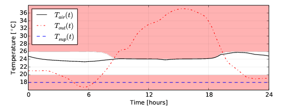
Fig. 9.30 Optimal room air temperature (black line), thermal discomfort zone (red area), outside temperature (red dotted) and supply air temperature (blue dashed).

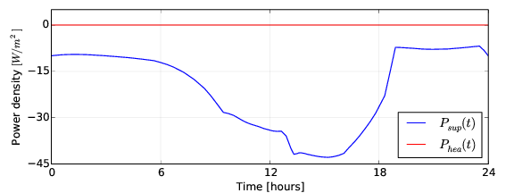
Fig. 9.31 Optimal cooling and heating power provided by the HVAC system through the VAV box.

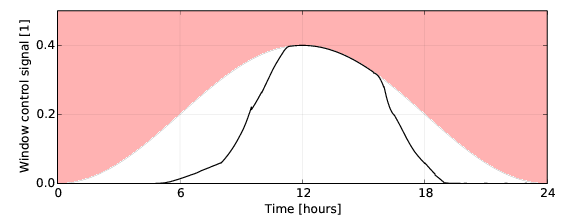
Fig. 9.32 Optimal control signal for the blind (black line).

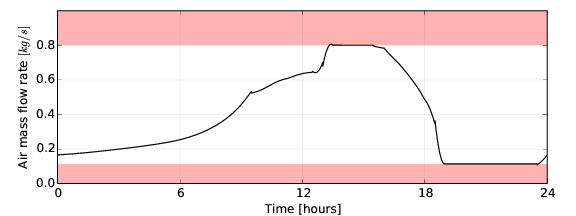
Fig. 9.33 Optimal supply air mass flow rate. The red areas indicate the infeasible regions.

Nelder-Mead algorithm: The blue lines in Fig. 9.35 show the optimal cooling load computed during successive iterations of the Nelder-Mead algorithm. Each line corresponds to a different penalty function multiplier \(\mu_i\), with the bold line being the final optimal solution. Fig. 9.34 shows a similar plot for the resulting optimal zone air temperature. As \(\mu_i\) increases, the solutions converge towards an optimal trajectory that satisfy the constraints.

Comparison: Both algorithms converge to solutions that minimize the energy consumption with a similar strategy. The strategy is to maintain the zone temperature close to the upper boundary of the thermal comfort zone during the peak hours. Both algorithms compute an optimal solution that reaches a maximum cooling power density of approximately \(45 \, \mathrm{W/m}^2\) around 4 PM. The trajectories computed by the two algorithms are different because of the different discretization mechanisms, implementations of the cost and constraint functions, and the numerical methods. The optimized total energy consumption \(E(t_f)\) is \(15.721 \, \mathrm{kWh/day}\) and \(16.543 \, \mathrm{kWh/day}\) for the optimization with the collocation and Nelder-Mead method, respectively. Hence, the collocation methods reduces the cost by an additional \(5.2\%\).

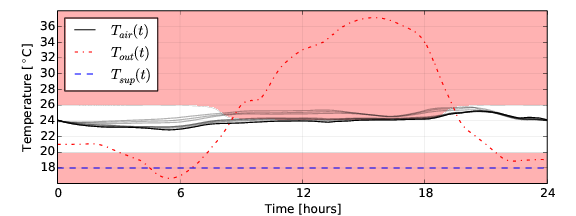
Fig. 9.34 Resulting optimal zone air temperature (black line) and its successive approximations for different values of the penalty function multiplier \(\mu_i\) (gray lines).

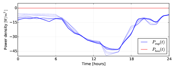
Fig. 9.35 Optimal cooling power provided by the HVAC system through the VAV box (blue line) and its successive approximations for different values of \(\mu_i\) (light blue lines), and optimal heating power provided by the VAV box (red line).

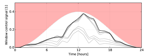
Fig. 9.36 Optimal control signal for the blind (black line) and its successive approximations for different values of \(\mu_i\) (gray lines).

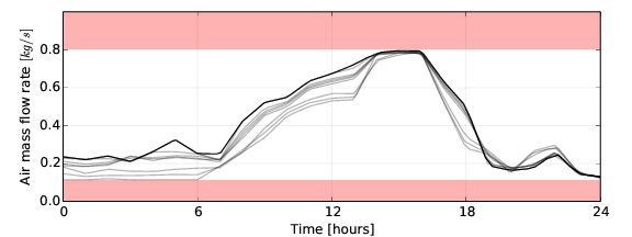
Fig. 9.37 Optimal supply air mass flow rate (black line) and its successive approximations for different values of \(\mu_i\) (gray lines). The red areas indicate the infeasible regions.

Table 9.1 and Table 9.2 show the statistics of the two optimization methods. Despite the fact that the optimization problem solved with the collocation method is larger and has a finer temporal resolution, it was solved approximately \(2,200\) times faster than the problem solved using Nelder-Mead.

Table 9.1 Statistics of the collocation-based optimization method.

Number of variables	10385
Number of equality constraints	9953
Number of inequality constraints	1160
Number of Iterations	72
Initialization time	0.93 s
Solution time	6.79 s
Post-processing time	0.04 s
Total computing time	7.75 s

Table 9.2 Statistics of the simulation-based optimization method for different values of the penalty multiplier \(u_{i}\) and for the cumulative time of the whole optimization.

\(\mu_{i}\)	Computing time in [s]	Function evaluations	Iterations
0.150	2673	25033	447
0.225	1461	13605	242
0.337	1877	16853	300
0.506	2829	25033	447
0.759	2276	20773	370
1.139	1768	16517	294
1.709	1498	13829	246
2.563	1793	15957	284
3.844	1222	10805	192
Total	17401	15840	2822

9.4.4. Building simulation scenario for optimal design

This section describes a case study in which a design parameter optimization was applied to a Modelica building system model. The system model is based on the Annex 60 library and the Modelica Standard Library.

9.4.4.1. Description of the Scenario

The system model represents a two story residential building with \(120 \, \mathrm{m^2}\) floor area. It has a solar heating system and a backup heater. Figure Fig. 9.38 shows the Modelica model.

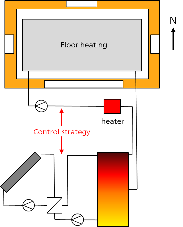
Fig. 9.38 Residential building with its solar heating system

The simulation model has to be fast because the parameter optimization can require hundreds of simulations.

The scenario is specified with following aspects:

9.4.4.2. Climate Locations

Two locations are used, San Francisco (relative warm climate during the heating period) and Chicago (very cold climate during the heating period).

9.4.4.3. User Behavior

A mean air change rate of 0.5 1/h is assumed. The air temperature setpoint profile for heating is 20°C. Internal heat sources are considered with a specific mean value of \(3 \, \mathrm{W/m^2}\). 50 percent is convective, and 50 percent is radiative.

9.4.4.4. Building Geometry and Thermal Properties

The building is a single family house with \(120 \, \mathrm{m^2}\) floor space. It has two identical stories and a flat roof as shown in Fig. 9.39.

The total thickness of the external walls in the reference case is 0.3 m, also for the base plate and the ceiling between the two stories. All inner walls have a thickness of 0.2 m. The roof thickness is 0.4 m.

The windows in the south façade have a width of 3 m and a height of 1.4 m. All the other facades (east, west, north) have windows with a smaller size of 1 m width and 1.4 m height. The height of the sill of all windows is 0.6 m. Because it is a theoretical model, doors are neglected. All rooms have the same size of \(15 \, \mathrm{m^2}\).

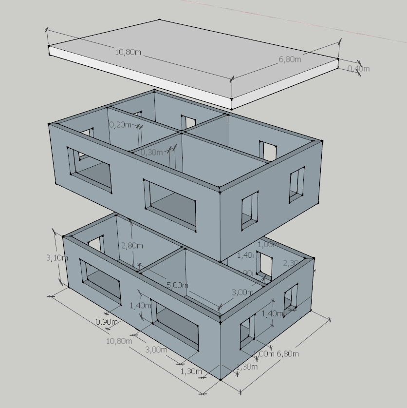
Fig. 9.39 Geometry of the two stories residential building

The materials listed in Table 9.3 were used for the specification of the opaque building elements.

Table 9.3 Materials of the opaque building elements.

Material	\(\rho \, [\mathrm{kg/m^3}]\)	\(c \, [\mathrm{J/(kg \, K)}]\)	\(\lambda \, [\mathrm{W/(m \, K)}]\)
Concrete	2,000	1,000	1.35
Insulation	30,0	1,000	0.04
Gravel	1,800	1,000	0.7

This leads to the U-values shown in Table 9.4.

Table 9.4 U-values of the opaque building elements.

Construction	\(U \, [\mathrm{W/(m^2 \, K)}]\)	Layers
External walls	0.35	20 cm concrete, 10 cm insulation
Floor	0.35	20 cm concrete, 10 cm insulation
Roof	0.34	20 cm concrete, 10 cm insulation, 10 cm gravel
Inner constructions	3.14	20 cm concrete

For the windows, the mean U-value of the panes and frame of the window is \(1.0 \, \mathrm{W/(m^2 K)}\) and the g-value for perpendicular irradiation is 0.6.

9.4.4.5. Energy Supply System

The energy supply system consists of a warm water heating system with floor heating. An additional solar thermal plant with a fixed azimuth angle of 0° and tilt angle of 30° generates thermal energy, which is fed into a solar storage. The specific mass flow rate through the solar collector field is \(40 \, \mathrm{kg/(m^2 \, h)}\).

The return flow of the heating loop is warmed up by the solar storage. If necessary, the backup system (heater) adds thermal energy to obtain the supply water temperature set point of 45°C.

9.4.4.6. Control System

The solar loop is controlled by a simple on/off controller. If the output temperature of the collector is 4 K above the temperature in the lowest layer of the solar storage, and the temperature is under 100 °C (in order to avoid boiling), then the solar pump is switched on until the temperature difference falls under 1 K. For the space heating, a two-way valve adjusts the water flow rate.

9.4.4.7. Implementation and Parametrization of the Scenario in Modelica

An implementation of the scenario, based on the Annex 60 library, the Modelica standard library and two models of the BuildingSystems library (a collector model and storage model, which are not present in the Annex 60 library) was realized. Fig. 9.40 shows the system model.

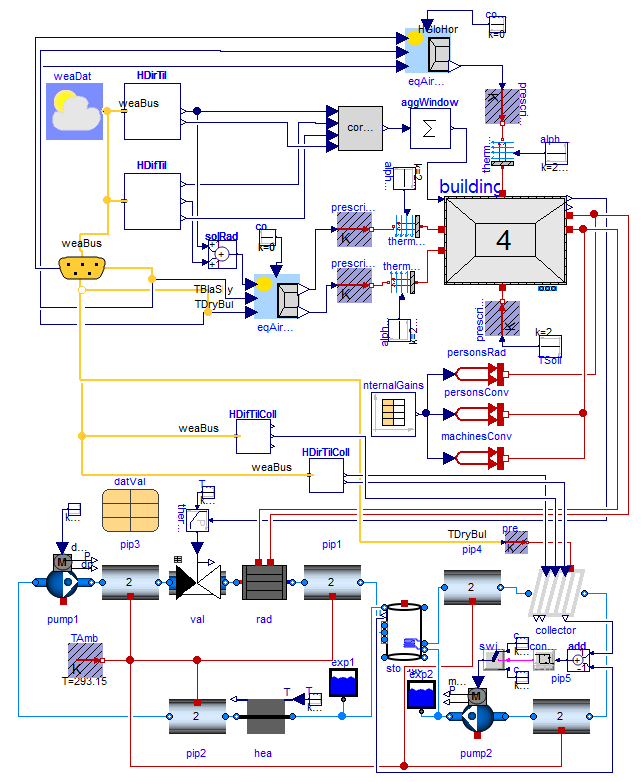
Fig. 9.40 Modelica model of the scenario.

The parameterization of the low-order building model was performed using the TEASER tool (https://github.com/RWTH-EBC/TEASER).

9.4.4.8. Optimization Problem

The following parameters were varied during the optimization:

• The thickness of the insulation of the exterior walls (from 6 cm to 30 cm),
• the volume of the solar storage (from \(1 \, \mathrm{m^3}\) to \(40 \, \mathrm{m^3}\)), and
• the collector area (from \(1 \, \mathrm{m^2}\) to \(40 \, \mathrm{m^2}\)).

The cost function consisted of components for labor and material costs for the insulation \(C_{ins}\), component and installment costs for the thermal collectors \(C_{col}\), component cost for the solar storage \(C_{sol}\) and energy cost for the needed backup energy \(C_{bac}\). An additional penalty factor \(C_{pen}\) considers a desired solar covering rate of the solar heating system:

\[Cf = C_{col} + C_{sto} + C_{ins} + C_{hea} + C_{pen},\]

where

\[C_{col} = \frac{200 \, A_{col}}{\tau{col}},\]

\[C_{sto} = \frac{1649.81 \, V_{sto}^{-0.464} \, V_{sto}}{\tau_{sto}},\]

\[C_{ins} = \frac{A_{ext} \, (2.431 \, d_{ins} \, 100.0 + 87.35)}{\tau_{ins}},\]

\[C_{bac} = r \, Q_{bac},\]

and

\[C_{pen} = p \, (SF_{set} - SF),\]

where \(\tau\) is the expected life time. Parameter optimizations with a energy prices \(r\) of 8 Euro cent per kWh and a penalty factor \(p\) of 0 Euro and 1,500 Euro were performed. A desired solar covering rate of \(SF_{se} = 0.5\) was assumed. The life time was assumed to be 20 years for the solar collector \(\tau_{col}\), 20 years for the solar storage \(\tau_{sto}\) and 30 years for the insulation \(\tau_{ins}\).

Because the optimization of the solar heating system has to be considered as a seasonal problem, each simulation run was performed over 2 years simulation time, where only the second year was evaluated for the cost function. The simulation starts from 1st of July with a start temperature for the solar storage of 60°C for the entire water volume. All optimization runs were initialized with an insulation thickness of 0.1 m, a solar collector area of \(20 \, \mathrm{m^2}\) and a volume of the solar storage of \(10 \, \mathrm{m^3}\).

The optimization problem was solved with GenOpt, using the Particle Swarm algorithm in combination with the General Pattern Search algorithm. Dymola 2017 was used to evaluate the cost function.

9.4.4.9. Optimization Results

The colder climate of Chicago leads to a larger insulation thickness of 15 to 20 cm in comparison to San Francisco, where 6 to 7 cm insulation are optimal. If the penalty factor is set to 1,500 Euro, then the thickness of the insulation is increasing at the colder location and decreasing at the warmer location, as shown in Fig. 9.41.

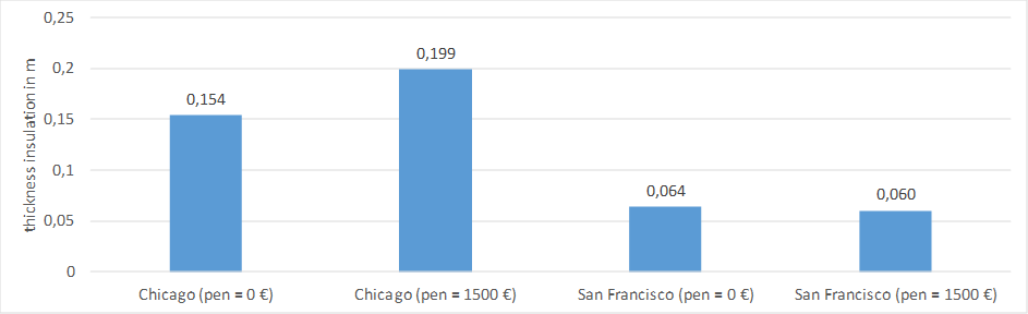
Fig. 9.41 Optimized insulation thickness for Chicago and San Francisco

A pure economic optimization (penalty factor = 0 Euro) leads to a solar coverage rate of 8.5 percent for Chicago and 19.6 percent for San Francisco, as shown in Fig. 9.42. With a penalty factor of 1,500 Euro, for both locations the solar coverage rate is about 50 percent, which minimizes the penalty term.

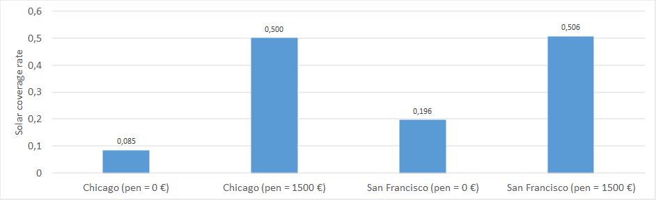
Fig. 9.42 Optimized solar coverage rate for Chicago and San Francisco.

The colder climate of Chicago causes a larger collector area than in San Francisco. If the penalty factor set to 1,500 Euro, then the collector area is drastically increased to reach the desired solar coverage rate, as shown in Fig. 9.43.

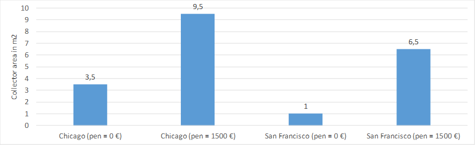
Fig. 9.43 Optimized volume solar storage for Chicago and San Francisco.

The optimized volume of the solar storage is \(1 \, \mathrm{m^3}\), except for Chicago (about \(30 \, \mathrm{m^3}\)) if the penalty factor of 1,500 Euro is applied. A seasonal storage of solar energy from the summer for the heating period with a large storage volume is a precondition to reach the desired solar coverage rate, as shown in Fig. 9.44.

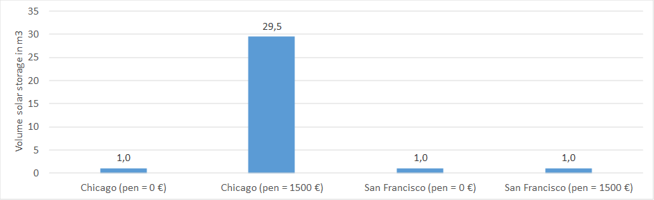
Fig. 9.44 Optimized volume solar storage for Chicago and San Francisco

Fig. 9.45 shows that the required backup energy in Chicago is 6 to 8 times higher than in San Francisco.

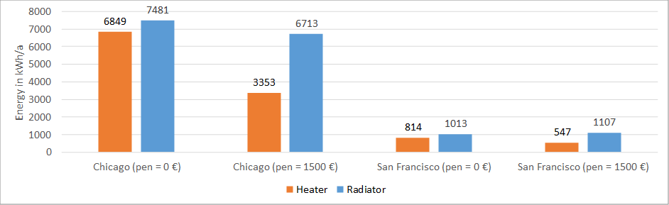
Fig. 9.45 Optimized thermal energies for Chicago and San Francisco

9.4.4.10. Computation Time

A single simulation run over two years took 33 seconds. GenOpt required between 25 minutes and 50 minutes.

9.5. Summary

The nine case studies from seven countries of Activity 2.1 have illustrated that Modelica building libraries are able to cover a wide range of building design and building optimization problems.

The authors of the case studies mentioned the following main advantages of Modelica: First, the modular approach of Modelica enabled them to model building systems at various levels of detail. Temporal and spatial resolution could be increased where needed to address a particular design question while abstracting other parts of the model using simplified equations. Second, Modelica’s object-orientation and encapsulation through standardized connectors for heat flow and fluid flow allowed collaborative development in which sub-models of complex building systems were configured by different modelers and subsequently combined to form a system model. Third, missing models could be added quickly, either through new implementations, through combinations of existing models, or through use of base classes that implement conservation equations. Fourth, models of different domains such as heat transfer, fluid flow, electrical systems and control systems could be combined graphically to form an integrated model. The main reported drawback of Modelica was that annual simulations can be time-consuming if detailed HVAC models are combined with multi-zone building envelop models. This is largely due to the solvers that are currently implemented in the Modelica simulators. As Modelica is translated to efficient C-code (see Section 5.3.4), this is not an inherent problem of Modelica, but rather a questions of what solvers to use as users simulate ever larger models. To obtain fast simulations, component parameters have to be adjusted and the right solver and its tolerance have to be chosen in the Modelica simulation tools [JWH15]. Moreover, detailed control algorithms can slow down the simulations performance, in particular if they generate many events. Addressing these problems is an active field of research, see for example Section 5.2.

Two examples could demonstrate the application of optimal design and optimal control problems based on Modelica libraries: A multi-criteria parameter optimization of PV cooling systems for residential buildings and a non-linear optimal control problem for the HVAC and facade control in a thermal zone. For the latter, the computer algebra conducted by the Modelica tool when it constructed the optimization problem, based on the declarative model formulation, led to 2,200 times faster optimization compared to a derivative free optimization method that simply evaluated the cost function iteratively.

A final building simulation scenario for optimal design summarizes the work of Activity 2.1: A parameter optimization method was exemplary applied to a Modelica building system model that couples a solar thermal system to a simplified building model. This building system model is almost entirely composed of components from the Annex 60 library and the Modelica standard library. A two-year simulation of this model took half a minute. Two optimization variants that optimize life cycle cost using weather data for a moderate climate and a very cold climate were performed.