5. Activity 1.1: Modelica

This chapter provides an overview of Modelica, gives an introduction with pointers to further literature about its capabilities, and presents the Modelica Annex60 library that has been developed within the IEA EBC Annex 60. The library is available from http://www.iea-annex60.org/releases/modelica/1.0.0/Annex60-v1.0.0.zip. The models are documented at http://www.iea-annex60.org/releases/modelica/1.0.0/help/Annex60.html. They will be further developed within the IBPSA Project 1 at https://github.com/ibpsa/modelica-ibpsa.

5.1. Introduction

Modelica is an object-oriented equation-based modeling language. The language has been developed to support design and operation of complex engineered systems that are governed by differential equations, algebraic equations, time- and state events. It is now used in various industrial sectors such as automotive, aerospace, electrical engineering, power plants, robotics, buildings and district energy systems.

At the time of this writing, more than 70 free open-source and commercial Modelica libraries were available, see for example https://modelica.org/libraries and http://impact.github.io/#/all. The Modelica Standard Library version 3.2.1, which is the official library of the Modelica Association, contains about 1500 models, blocks and functions, covering most engineering domains.

The goal of the Annex 60 library development is to provide well documented, vetted and validated open-source Modelica models that will serve as the core of future building and district energy simulation programs.

5.2. Literature Review

Modelica origins in the PhD thesis of Hilding Elmqvist in 1978 at the Department of Control, Lund University, under the supervision of Karl Johan Åström [Elm78]. In [Elm14], Elmqvist gives a perspective on the Modelica evolution which is summarized as follows: In his PhD thesis, Elmqvist designed the DYnamic MOdeling LAnguage Dymola, which contained a class object for object-oriented modeling and a structured feature to describe interaction between submodels. In Spring 1996, discussions started to unify the modeling languages Dymola, Omola, NMF and Allan. In Fall 1996, the first design meeting was held as Elmqvist realized that it was time for a global unified language design initiative. The primary reason was that modeling requires reuse of stored knowledge and hence a standard language, rather than the various tool vendors inventing their own language and a new language being created for every PhD thesis on modeling. In 1997, after one year of design, Modelica 1.0 was released. The first version of Dymola that supported Modelica was released in 1999 and three years later the first open-source implementation OpenModelica followed [FAB+02b].

In the buildings community, the use of equation-based languages has its origin in the energy simulation program ENET [LS82][STLL84], which provided the foundation of the SPANK or SPARK program [SBEW86][SBN89][BEWS93]. In 1989, Sahlin and Sowell [SS89] introduced an equation-based language called Neutral Model Format (NMF) which is used in the commercial software IDA/ICE [BBE+99]. In 1993, Klein introduced the equation-based Engineering Equation Solver EES [Kle93].

Felgner et al. [FAB+02a] reported in 2002 the earliest applications of Modelica for building energy simulation [Mer02], which led to the ATPlus library [FAB+02a] which no longer seems to be developed. In 2005, Nytsch-Geusen et al. presented a hygrothermal building model [NGNHH05]. In 2004, development of a proprietary Modelica library for building and HVAC system simulation started at the United Technology Research Center [Wet06b][Wet06a]. In 2007, Wetter started at LBNL the development of the open-source Modelica Buildings library [WHMS08][Wet09][WZNP14]. Also in 2007, Müller started to develop the model library AixLib for building and urban energy systems at RWTH Aachen University [BM10][FCL+15]. This work was based on his first activities at TU Berlin to model active building components in Modelica [HHTM05]. In 2010, Baetens et al. started at KU Leuven the development of IDEAS, a library for Integrated District Energy Assessment Simulations [BDCVR+12][BDCJ+15]. In 2012, Nytsch et al. presented the Modelica BuildingSystems library developed at UdK Berlin [NGHLR12].

Between 2012 to 2014, the AixLib, BuildingSystems and IDEAS libraries were made open-source to facilitate collaboration within the IEA EBC Annex 60. With the AixLib, Buildings, BuildingSystems and IDEAS libraries, four open-source libraries for building and district energy systems became available; however, due to different design choices and modeling principles, combining models from these libraries was cumbersome if not impossible for most users. Furthermore, because the libraries used different conventions and implementations, sharing development effort was not possible prior to the Annex 60, thereby wasting development resources. Therefore, within Annex 60, the design choices of these libraries were harmonized, models were made compatible, and a common core of a Modelica library, the Annex60 library, has been developed [WFG+15]. All four of these libraries are now based on the collaboratively developed Annex60 library whose goal is to provide a well-documented, vetted and validated open source Modelica library that serves as the core of future building simulation programs.

In addition to these open-source libraries, various commercial and proprietary libraries have been developed. In 2005, Modelon presented the AirConditioning library [TEP05] for detailed steady-state and dynamic modeling of vapor compression cycles, and TLK Thermo presented a similar library as part of the TIL suite [GKRT10]. Since 2009, XRG develops and distributes the HVAC library and HumanComfort libraries [ME09]. In 2012, ITI, EA Systems, Honda and TU Dresden introduced the GreenBuilding library [USM+12]. In 2014, Électricité de France presented the BuildSysPro library [PKL14].

Various literature compares equation-based and procedural modeling languages. Sahlin [Sah96] reports that developing a simulation model in the equation-based modeling language NMF [SS89] was about three times faster than it was in the BRIS simulation program [Bro90], but the computation time in BRIS was three times faster. Sahlin et al. [SEG+04] compared the computation time of IDA ICE with EnergyPlus. In their numerical experiments, IDA ICE required approximately half the computation time that was required by EnergyPlus for a three zone building with natural ventilation and twice the computation time in an initial experiment for a 53 zone building without natural ventilation. In the latter experiments, the COMIS airflow program was not included in EnergyPlus. Sowell and Haves [SH01] compared the computation time of SPARK and HVACSIM+ for a variable air volume flow system that serves six thermal zones. They report that SPARK computes about 15 to 20 times faster than HVACSIM+ and attribute the faster computation to SPARK’s graph decomposition and cut set reduction. Wetter et al. [WHMS08] compared the SPARK solver with Dymola for a variable air volume flow system with five zones and concluded that they have comparable computing time. Wetter and Haugstetter [WH06] compared computing time in TRNSYS and the Modelica environment Dymola. TRNSYS simulated about three to four times faster, which most likely was due to the time series representation used in TRNSYS for the conduction heat transfer calculation. Jorissen et al. [JWH15] show how model and solver knowledge can lead to simulation times that are two orders of magnitude lower for large Modelica models when using explicit solvers instead of implicit solvers.

Also, decreasing the computing time for large Modelica models through changes in the Modelica translators and numerical methods is an active area of development, see for example [MBKC13][FBC+14][Cas15][BBCK15][BRC16][CR16][OE17][BCB17][JHB17].

To compare the labor time for model development, Wetter [Wet11b] compared the development time and, as development time often scales with code size, he also compared for cross comparison the code size for models in Fortran, C/C++ and Modelica. Their development time comparison indicates a five to ten times faster development through use of Modelica rather than C++ for the C++ multizone building model of BuildOpt [Wet05]. This translated to about one year of labor savings. The Modelica implementation required 6,000 lines of code while the C++ implementation required 24,000 lines. A similar reduction in labor time was observed for a small heat transfer problem that was independently implemented in Fortran and in Modelica by three engineers who were familiar with both languages. See Fig. 5.1.

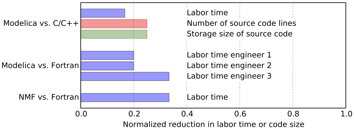
Fig. 5.1 Comparison of relative reduction in labor time and code size for equation-based vs. procedural programming languages.

5.3. What is Modelica

This section gives an overview about the main capabilities of Modelica. The intent is to familiarize the reader with the ideas of the Modelica language and explain how Modelica models are converted to simulation code. While most users will use existing Modelica component models from a library, this section also gives some background information that helps understanding the principles of the language.

Modelica is an equation-based, acausal, object-oriented modeling language that is designed for component-oriented modeling of dynamic systems. Models are described by differential equations, algebraic equations and discrete equations. Using standardized interfaces, the mathematical relations of a problem between its interface variables are encapsulated in a model, which can be represented graphically by an icon. The interface variables of multiple models can be graphically connected with each other in a graphical model editor, without requiring any notion of what is input and what is output of a model. This encapsulation together with the standardized acausal model interface facilitates model reuse and model exchange. Since Modelica is a standardized language, models can be shared and exchanged by a large user community.

To realize such a flexible modeling environment, the Modelica language embodies the object-oriented modeling paradigm, a term that was coined by Elmqvist [Elm78] and summarized by Cellier et al. [CEO95] as follows:

Encapsulation of knowledge:  The modeler must be able to encode all knowledge related to a particular object in a compact fashion in one place with well-defined interface points to the outside. Topological interconnection capability:  The modeler should be able to interconnect objects in a topological fashion, plugging together component models in the same way as an experimenter would plug together real equipment in a laboratory. This requirement entails that the equations describing the models must be declarative in nature, i.e., they must be acausal. Hierarchical modeling:  The modeler should be able to declare interconnected models as new objects, making them indistinguishable from the outside from the basic equation models. Models can then be built up in a hierarchical fashion. Object instantiation:  The modeler should have the possibility to describe generic object classes, and instantiate actual objects from these class definitions by a mechanism of model invocation. Class inheritance:  A useful feature is class inheritance, since it allows encapsulation of knowledge even below the level of a physical object. The so encapsulated knowledge can then be distributed through the model by an inheritance mechanism, which ensures that the same knowledge will not have to be encoded several times in different places of the model separately. Generalized Networking Capability:  A useful feature of a modeling environment is the capability to interconnect models through nodes. Nodes are different from regular models (objects) in that they offer a variable number of connections to them. This feature mandates the availability of across and through variables, so that power continuity across the nodes can be guaranteed.

The following subsections describe the approaches that are used in Modelica to realize this object-oriented modeling paradigm.

5.3.1. Acausal Modeling

5.3.1.1. Physical Connectors and Balanced Models

A tenet of Modelica is that each component should represent a physical device with physical interface ports called connectors. To accomplish this, Modelica requires models to be balanced. Casually expressed, a model is balanced when the number of its equations equals the number of its variables. A more rigorous definition can be found in [OOME08]. Models interact with other models through connectors. The connectors of a model contain all variables required to uniquely define the boundary conditions of the model.

The Modelica Standard Library implements connectors for various domains, such as heat transfer, fluid flow, electrical and translational systems. These connectors declare the interfaces of the models. Table 5.1 shows different connectors and their variables, which are either potential, flow or stream variables. Potential variables are the driving force for a flow, and hence examples are voltage \(V\), position \(x\), temperature \(T\), and pressure \(p\). The associated flow variables are current \(I\), force \(F\), heat flow rate \(\dot Q\) and mass flow rate \(\dot m\). Thermofluid flow systems are a special case because the mass flow rate carries properties such as specific enthalpy \(h\), mass fractions \(X\) and trace substance concentrations \(C\). These properties therefore change depending on the flow direction. Hence, these are stream variables, and are, for numerical performance, treated in Modelica in a unique way [FCO+09a].

When connectors are connected with each other, Modelica automatically generates equations that equate the potential variables. For example, connecting \(n\) connectors of heat flow components \(c_i\), for \(i \in \{1, \ldots, n\}\), results in all \(c_i\) having the same temperatures at the connection points, e.g., \(c_1 \, T = c_i \, T\), for all \(i \in \{1, \ldots, n\}\). Furthermore, for the electrical, translational and heat flow domain, the sum of the flow variables is set to zero. For example, for the above heat flow components, Modelica will generate the equations \(0 = \sum_{i=1}^n c_i \, \dot Q\). Thermofluid flow components are different because the mass flow rate \(\dot m\) carries the fluid properties \((h, C, X)\). To allow connecting multiple fluid connectors, Modelica uses so called stream-connectors [FCO+09a]. This allows Modelica to generate for connected thermofluid flow components the equations for conservation of mass \(0 = \sum_{i=1}^n c_i \, \dot m\). For the properties that are carried with the flow, Modelica generates the equations

(1)\[\chi_{mix} = \frac{\sum_i \dot m^+_i \, \chi_i}{\sum_i \dot m^+_i},\]

where \(\chi\) is any of the conserved quantities \((h, C, X)\) and \(\dot m^+_i = \max(0, \dot m)\).

Table 5.1 Physical connectors from the Modelica Standard Library.

Domain	Potential	Flow	Stream
Electrical	\(V\)	\(I\)
Translational	\(x\)	\(F\)
Heat flow	\(T\)	\(\dot Q\)
Thermofluid flow	\(p\)	\(\dot m\)	\(h\), \(X\), \(C\)

These rules allow to connect one or multiple components to any physical port. For example, if a heat flow port is unconnected, then no equation for its temperature is introduced, and the heat flow rate across this port is set to zero, thereby rendering the port as an adiabatic boundary condition. Whether a port variable is an input or an output to the model is determined when the model is translated. Hence, models impose no causality on the connector variable. This property allows to reuse, for example, a model for one-dimensional steady-state heat conduction for situations where both port temperatures are known and the heat flow rate at the ports need to be computed, or where one port temperature and heat flow rate are known and the other port temperature and heat flow rate needs to be computed.

This encapsulation of balanced models with acausal physical connectors enables a graphical, input-output free model construction, as we will see later in this section. In a schematic model diagram of a physical system, icons correspond to actual components or subsystems and encapsulate the equations that define the physics of the subsystem. Lines between the icons impose the port equations to conserve flow and to equate state variables, or they may propagate signals in a control system. Because these connectors are standardized, models from different libraries can be connected with each other, thereby allowing users to use models from various domains and libraries within one system model.

5.3.1.2. Illustration of a Simple Model

We will now illustrate how a simple heat flow component is built using the heat flow connector of the Modelica Standard Library. This connector is implemented by the following lines of Modelica code:

partial connector HeatPort
    "Thermal port for 1-D heat transfer";
  SI.Temperature T "Port temperature";
  flow SI.HeatFlowRate Q_flow "Heat flow rate";
end HeatPort;

On line 4, the type prefix flow declares that Q_flow is a flow variable and hence need to be summed to zero as explained above. This connector can then be instantiated to define the interface with the outside of the model in a one-dimensional heat transfer element with no energy storage. In Modelica’s thermal library, such a heat transfer element is implemented as follows:

partial model Element1D
  "Partial heat transfer element with two HeatPorts"
  SI.HeatFlowRate Q_flow
    "Heat flow rate from port_a->port_b";
  SI.TemperatureDifference dT "port_a.T-port_b.T";
 public
  HeatPort port_a "Heat port a";
  HeatPort port_b "Heat port b";
 equation
  dT = port_a.T - port_b.T;
  port_a.Q_flow = Q_flow;
  port_b.Q_flow = -Q_flow;
end Element1D;

Lines 3 to 5 contain the declaration of the variables \(\dot Q\) and \(\Delta T\) that are typically computed in a one dimensional heat transfer element. Lines 7 and 8 instantiate the HeatPort connector to expose to the outside of this model the port temperatures port_a.T and port_b.T, as well as the port heat flow rates port_a.Q_flow and port_b.Q_flow. The equations on line 10 to 12 define the relationships among the variables of the two HeatPort connectors and the variables of the partial model Element1D. Note that Element1D does not declare a relation between the heat flow rate and the temperatures, as this relation is different for conduction, convection or radiation. Because this relation is not specified, the model is declared partial to indicate that it can be extended by other models to refine its implementation, but that it cannot be instantiated directly as it does not define how temperature and heat flow rate are related. To implement a thermal conductor, the above partial model can be extended as follows:

model ThermalConductor
  "Lumped thermal element
   transporting heat without storing it"
  extends Interfaces.Element1D;
  parameter SI.ThermalConductance G
    "Constant thermal conductance";
equation
  Q_flow = G*dT;
end ThermalConductor;

This thermal conductor model can then be encapsulated in a graphical icon using drawing elements that are part of the Modelica language standard, and hence, can be interpreted by different Modelica modeling environments. By using a different parameter declaration on line 5 and a different equation on line 8, the semantics can be changed to represent other one-dimensional heat transfer elements such as a model for long-wave radiation between two surfaces. Note that the above code is not pseudo-code, but rather a complete implementation of a heat conductor in the Modelica language, except for the optional graphical annotations that will be explained in the next section. Note that in the implementation above, the model developer only declared the variables and the constraints between heat flow rate and temperatures. Whether the model will solve for the heat flow rate or for a port temperature will be determined by a code generator that analyzes the overall simulation model in order to determine a numerically efficient sequence of computations, as we will show in Section 5.3.4.

5.3.1.3. Graphical Encapsulation

Creating, changing and understanding reasonably large system models without a graphical model editor would be very cumbersome if not impossible. To be able to use models in different graphical model editors, Modelica also standardizes graphical elements such as lines, circles and colors that can be used to graphically render an icon which encapsulates the model. In graphical editors, these icons can be opened to see the actual model implementation, and the icons can be used to graphically assemble components to build system models. Fig. 5.2 shows how the above heat conductor can be used to compute the heat flow rate for a time-varying and a constant temperature boundary condition on the left and right, respectively.

Fig. 5.2 Thermal conductor with varying temperature boundary conditions.

5.3.1.4. Object-Oriented Modeling

Object-oriented modeling allows reusing common functionalities across different models. Duplication of code which would make it difficult to correct coding errors throughout a large library of models when code is copied to different models. In the Annex60 library, object-orientation is extensively used to implement heat and mass balances of thermofluid flow components. It is also used, for example, to implement two-way control valves, which we will use here to explain the principle of object-oriented modeling.

Two-way valves can be characterized by an opening function

(2)\[ \varphi(y) = \frac{k(y)}{K_v},\]

where \(y \in [0, \, 1]\) is the control input, \(k \, \colon \, [0, \, 1] \to \Re\) is the flow rate divided by the square root of the pressure drop and \(K_v = k(1)\) characterizes that flow rate for a fully open valve. For a valve with linear opening characteristic, \(\varphi(y) = l + y \, (1-l)\), where \(l\) is the leakage of the closed valve, whereas for an equal percentage valve, the function \(\varphi(\cdot)\) is more complicated. To share code that is common among these valves, we can implement a base class such as

partial model PartialTwoWayValveKv
  "Partial model for a two way valve using Kv"
  extends BaseClasses.PartialTwoWayValve;

equation
 k = phi*Kv_SI;
 m_flow=BaseClasses.FlowModels.basicFlowFunction_dp(
   dp=dp, k=k, m_flow_turbulent=m_flow_turbulent);
 // ... (other code omitted for brevity)

Now, we can implement the valve with linear opening characteristics by extending this base class and assigning the function \(\varphi(\cdot)\) as follows:

model TwoWayLinear
  "Two way valve with linear flow characteristics"
  extends BaseClasses.PartialTwoWayValveKv(
    phi=l + y * (1 - l));
 // ... (other code omitted for brevity)
end TwoWayLinear;

Similarly, the valve with equal percentage opening characteristics can be implemented as

model TwoWayEqualPercentage
  "Equal-percentage two-way valve"
  extends BaseClasses.PartialTwoWayValveKv(
    phi=BaseClasses.equalPercentage(y, R, l, delta0));
  parameter Real R=50
    "Rangeability, R=50...100 typically";
  // ... (other code omitted for brevity)
end TwoWayEqualPercentage;

where the function BaseClasses.equalPercentage implements the opening characteristics.

This object-inheritance has various benefits. For users, if they understand what physics is implemented in the base class, for example that the valve linearizes the pressure drop calculations at very small flow rates, then they know that this applies to both valves. For a developer, if a new capability need to be implemented, such as a heat loss of the valve, then this can be done in the base class and will be automatically propagated to both valves models. This is also useful for users that build system models from existing component models. For example, in a variable air volume (VAV) flow system, each VAV damper likely has the same controller. Hence, the user can implement the controller in one object and instantiate it for each VAV damper. Should the control law require changes, then this can be done at a central place and the change be propagated to all instances of this controller.

5.3.1.5. Hierarchical Modeling

Hierarchical modeling supports keeping a well-defined and visually accessible model structure and helps manage complexity. This is aligned with the fact that physical problems are often analyzed by disaggregating them into several parts. Using hierarchical modeling allows having the same view within simulation models.

Consider for example modeling the thermal mass of a building. Standard workflow encompasses disaggregating the building into several thermal zones. In our fictive case, we consider two thermal zones (Fig. 5.3). Each of these thermal zones encompasses a number of wall elements representing e.g. exterior walls, interior walls and floor plates. These wall elements interact with each other by radiative heat exchange and via convective heat exchange through the indoor air volume. Each wall element in turn encompasses the description of heat transfer and heat storage effects, in our case described by thermal resistances and capacities.

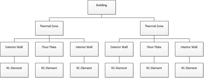
Fig. 5.3 Hierarchical structure of a thermal building model with levels for building, thermal zones, wall elements and RC-elements.

Using hierarchical modeling approaches in Modelica, each level of thermal mass modeling can be created by connecting sub-models that represent lower levels. In this way, each level takes care of modeling the interactions between the sub-models.

Refering to the system given in Fig. 5.3, the uppermost level is the building itself. At this level, we instantiate two thermal zones, using reduced order models for thermal zones with three wall elements:

model Building
  "Illustrates the use of hierarchical modeling"

  RC.ThreeElements thermalZoneOne(...)
  "Thermal zone one";
  RC.ThreeElements thermalZoneTwo(...)
  "Thermal zone two";

The visualization in the schematic diagram editor shows at the building level both thermal zones as simple icons without revealing any insights such as their sub-models. These insights become only visible on the thermal zone level as shown in Fig. 5.4. This level implements the interactions of the walls, e.g., the radiative heat exchange. It also instantiates wall elements for exterior walls, interior walls and a floor plate.

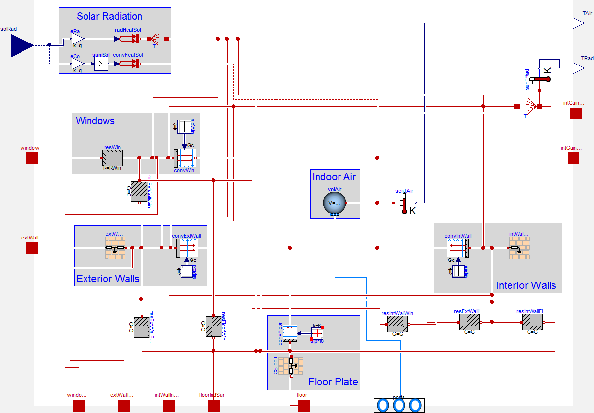
Fig. 5.4 Diagram view of a thermal zone model with three wall elements (exterior walls, interior walls and floor plate), windows and indoor air volume.

Looking into BaseClasses.InteriorWall, as shown in Fig. 5.5, reveals the actual implementation of resistances and capacities. These are connected in series using vectors of models to create a finite difference heat transfer model.

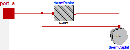
Fig. 5.5 Diagram view of a thermal network for interior walls, consisting of an array of thermal resistances and capacities.

5.3.1.6. Architecture-Driven Modeling

When evaluating different building systems, it is convenient to implement a system model of a base line, and then only declare how design variants differ from the base line. Modelica supports such modeling through architecture-driven modeling, which enables declaration of which models can be replaced with a different implementation. For illustration, consider a simple example in which we are interested in evaluating two different valves for a heat exchanger. One valve has linear opening characteristics, whereas the other valve has exponential opening characteristics. This can be accomplished by implementing a system model of the base case, which contains the valve with the linear opening characteristics. We can declare this, using the TwoWayLinear valve described above with the following code:

replaceable TwoWayLinear valve
  constrainedby BaseClasses.PartialTwoWayValveKv(
  redeclare package Medium = Medium,
  CvData=Buildings.Fluid.Types.CvTypes.Kv,
  Kv=0.65,
  m_flow_nominal=0.04)
  "Replaceable valve model”;

Here, we declared that the valve is of type TwoWayLinear (a two-way valve with linear opening characteristics) and it can be replaced by any other valve that uses (extends) the base class PartialTwoWayValveKv. The valve uses \(K_v\) data for the flow coefficient, with \(K_v = 0.65\) and a design mass flow rate of \(\dot m = 0.04 \, \mathrm{kg/s}\). These values are also applied to any valve that replaces this TwoWayLinear valve. Typically, such a model is part of a larger system model as shown in Fig. 5.6 in which the replaceable valve is graphically rendered by a gray box.

Fig. 5.6 Model with heat exchanger, feedback control and replaceable valve. The gray background rendered around the valve indicates visually that this model can be replaced by another implementation.

With the few lines of code below, which can be either entered in a textual editor or created from a graphical model editor, we can create a new model that is identical to the previous model except for the valve. The corresponding declaration is:

model EqualPercentageValve
  "Model with equal percentage valve"
  extends DryCoilCounterFlowPControl(
  redeclare Actuators.Valves.TwoWayEqualPercentage
    valve);
end EqualPercentageValve;

This allowed us to change the architecture of the system by replacing a model, while reusing everything else in the base case. In large systems that may have hundreds of models, such modeling is very convenient as it shows only what has changed from one version to another. Note that the replaced model can be another hierarchical system model, for example one can replace in a whole building simulation a heating plant with a gas furnace by a plant that uses a heat pump with a borehole heat exchanger.

5.3.2. Separation of Concerns

When implementing a model, a model developer typically writes computer code that implements functions, variable assignments, computing procedures, numerical methods and routines to obtain input. With Modelica, this is no longer needed, as it suffices to simply state the physical laws and the control algorithm that a model should obey. Therefore, Modelica requires only declaration of the physics and dynamics of a model. How to solve the equations, which variables to assign first, when to read input and update outputs etc. need not be specified. Thus, it is a modeling language, as opposed to an imperative programming language such as C/C++. The underlying design philosophy is to separate the concerns between modeling, simulation and other applications such as optimization or real-time simulation. In Modelica it suffices to implement a mathematical model of the system without having to specify how to solve the equations. The simulation program is automatically generated from the mathematical model using a Modelica translator that employs computer algebra as explained in Section 5.3.4. This allows for various target applications: For example, from a Modelica model, code can be generated for the following:

A conventional time-domain simulator:  that uses a classical ordinary differential equation solver, and optionally generate code for sequential or parallel computing [EMO14]. A discrete-event simulator:  that can handle order of magnitudes bigger models than classical ordinary differential equation solver [MBKC13]. A building automation system:  that imports control code in a standardized format [NW14]. An embedded real-time controller:  that may not have any hard disk for file input and output. A web application:  in which the model is translated to JavaScript so it can run native in a web-browser [Fra14]. An optimization program:  that symbolically converts the model to a form that allows computing optimal control functions significantly faster than conventional optimization methods [WBN16].

Such a separation between mathematical model and executable application code is a critical underlying principle for a future modeling and simulation environment for building systems. By following this principle, it is possible to structure the problem more naturally in the way a human thinks, and not how one computes a solution.

5.3.3. Example Model

Fig. 5.7 demonstrates how a simple model can be constructed using components from the Annex 60 library. The model is available in the Annex60 library as Annex60.Fluid.Examples.SimpleHouse. It consists of a simple building, a heating system and a ventilation system, with both systems including a controller. The building model consists of a wall, an air volume and a window. The wall is represented using a simple model consisting of a single heat capacitor and a heat conductor. The zone air is modeled using a control volume with mixed air, which is connected to the wall using a thermal resistor which represent the convective heat transfer. The window is modeled using a component that injects heat onto the wall. Boundary conditions are the outside temperature of the wall and the solar irradiation on the window.

The heating system consists of a radiator, a pump and a heater as illustrated in the bottom of the figure. The heater thermal power is controlled using an on/off controller with hysteresis that tracks a set point for the zone air temperature.

To ventilate or cool the room, a ventilation system is modeled that consists of a heat recovery unit, a fan, a cooling device and a damper. The fan applies a constant pressure difference over the damper. The damper position is modulated by a proportional controller to provide more air if there is a need for cooling.

To build the model, each individual component model was dragged from the component library, placed on the schematic editor window, and connected to other components much like physical components. Model parameters like the pump mass flow rate were set by double-clicking on the respective component, which opened a parameter window. More detailed building models may be implemented using one of the libraries that extend the Annex60 library and are listed at Section 5.4.2.

Fig. 5.7 Modelica system model SimpleHouse as rendered by a Modelica graphical model editor.

5.3.4. Model Translation

The translation of a Modelica model into a simulation program is a fully automated process. When translating a model, symbolic processing is important to reduce computing time since many building system simulation problems lead to large, sparse differential algebraic equation systems (DAE systems). Symbolic processing is typically used to reduce the index of the DAE system and to exploit sparsity. The following methods are typically used in Modelica simulation environments. To solve a DAE system with ordinary differential equation solvers, the index of the DAE is reduced using the algorithm of Pantelides [Pan88]. Next, to exploit the sparsity of the model, Modelica translators generally convert the coupled system of equations to block lower triangular form, by changing the equation order. This process is called block lower triangularization and is discussed in detail by Duff [DER89]. A simple example is as follows: Consider the system of equations

(3)\[\begin{split}\dot Q(t) & = T_1(t)^4 - T_2(t)^4, \\ f_1(t) & = T_1(t)^4, \\ f_2(t) & = T_1(t)^4 + T_2(t)^4,\end{split}\]

where \(f_1, \, f_2 \, \colon \, \Re \to \Re\) are known functions of time and \(T_1, T_2, \dot Q\) are unknowns. A naive implementation would solve directly a three-dimensional non-linear system of equations using a Newton solver. However, we can consider the incidence matrix whose columns are the independent variables and rows are the equations, as shown on the left of Table 5.2. In the incidence matrix, cell (i,j) contains an x if the independent variable i depends on the equation j.

Table 5.2 Incidence matrix prior to block lower triangularization.

Equation	\(T_1(t)\)	\(T_2(t)\)	\(\dot Q(t)\)
1	x	x	x
2	x
3	x	x

For this system, we can permute the rows so that all cells with an x are below the diagonal, as shown in Table 5.3.

Table 5.3 Incidence matrix after block lower triangularization.

Equation	\(T_1(t)\)	\(T_2(t)\)	\(\dot Q(t)\)
2	x
3	x	x
1	x	x	x

This shows that by rearranging the equations, we can solve sequentially

(4)\[\begin{split}f_1(t) & = T_1(t)^4, \\ f_2(t) & = T_1(t)^4 + T_2(t)^4, \\ \dot Q(t) & = T_1(t)^4 - T_2(t)^4.\\\end{split}\]

Finally, using computer algebra, these equations can be converted into the explicit assignment

(5)\[\begin{split}T_1(t) & = (f_1(t))^{1/4}, \\ T_2(t) & = (f_2(t) - T_1(t)^4)^{1/4} \\ \dot Q(t) & = T_1(t)^4 - T_2(t)^4,\end{split}\]

and hence no iterative solution is required.

After block lower triangularization, there may still be sets of equations that require a coupled iterative solution. In this situation, tearing can be used to break the dependency graph of equations and variables to further reduce the dimensionality of the coupled system of equations. The resulting coupled systems of equations are typically small but dense. Tearing can be done automatically or it can be guided by using physical insight with language constructs that can be embedded in a model library [EO94]. A simple example of tearing is as follows: Suppose we have an equation of the form

(6)\[0 = f(x),\]

for some \(x \in \Re^n\), with \(n > 1\), that can be written in the form

(7)\[\begin{split} L \, x_1 & = \hat f_1(x_2), \\ 0 & = \hat f_2(x_1, x_2),\end{split}\]

where \(L\) is a lower triangular matrix with constant non-zero diagonals. If this is the case, we can pick a guess value for \(x_2\), solve the first equation for \(x_1\), compute a new value for \(x_2\) from the second equation and iterate until \(x_2\) converges. As \(\hat f_1(\cdot)\) has fewer equations than \(f(\cdot)\), this often results in faster computation as the computing time of many numerical algorithms grows proportional to \(n^3\).

Fig. 5.8 from the Dymola 2016 user manual shows for a mechanical model with kinematic loops that consist of \(1,200\) equations how symbolic processing significantly reduces the dimension of the coupled systems of equations.

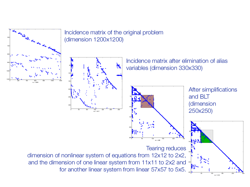
Fig. 5.8 Reduction of the dimension of the system of equations for the case of a mechanical model during the symbolic processing.

Finally, a further reduction in computation time can be obtained by symbolically inserting the discretization formula that represents the numerical integration algorithm into the differential-algebraic equation model, a process called inline integration that was introduced by Elmqvist et al. [EOC95].

5.3.5. Use of External Code

While the above model translation is powerful, there are situations where a human programmer can generate more efficient code. In the buildings domain, a typical example is the solution for partial differential equations for computational fluid dynamics. Partial differential equations often lead to repeating structures, such as a band-diagonal matrix, for which efficient solution algorithms or parallelization methods can be devised or that can simulate faster when parts of the computation is done on a graphical processing unit, see for example [ZC10]. For such situations, the Modelica language allows for the calling of C or FORTRAN 77 code, as well as compiled code. Using C code is for example used in the Buildings library to connect Modelica with Python, and compiled code is used to link code for computational fluid flow dynamics for indoor air simulation to the building model in [ZWT+16].

5.3.6. Debugging

When talking about debugging, users typically mean instruction-by-instruction execution of a program code. This makes sense for imperative programming languages such as C/C++, or for signal flow diagrams such as in Simulink, or in actor-based modeling such as in Ptolemy II. However, Modelica, except for the body of Modelica functions, has no notion for line-by-line execution. The equations are declarative. A tool can rearrange equations, invert them by changing variables on the left- and right-hand side or by doing other computer algebra before it generates code. Hence, the process of “simulating” a Modelica model is fundamentally different from simulating a model that is expressed in code such as C/C++, Java or Python. Consequently, debugging needs to be approached differently.

To explain how to debug declarative Modelica models, let us first stipulate that the code is translated correctly from Modelica to an executable language such as C/C++, but that the trajectories of the simulation are unexpected. Therefore, one debugs to verify what equations, not what variable assignment, may be wrong. This is often easiest by breaking up large models into small component models and test them individually. Through this process, wrong equations are often easy to detect by looking at the results of a simulation and comparing them to an analytical solution. This is also the reason why good model development should always include the implementation of small unit tests, preferably for different input signals for which the correct solution is known a-priori. Then, assembling models to form larger systems seldom introduces an error due to Modelica’s implementation of physical connectors and its requirements of models to be balanced, as described in the Section 5.3.1.1.

Debugging can also consist of understanding why a system model has large linear or nonlinear algebraic loops. In this situation, Modelica translators typically allow for the inspection of intermediate formats that are human-readable model representations after the symbolic manipulation but before generating C code. For example, an intermediate format can show which equations relate the inputs to the outputs and which equations require use of a linear solver or use of a nonlinear iterative solver.

Another purpose of debugging may be to reduce computing time. For this purpose, some simulation environments allow for running diagnostics on the model to see in what equations most of the computing time is spent, what variables dominate the error and the time step size control, and what logical tests produce events that can increase the computing time.

Furthermore, tools typically have intermediate formats and/or debuggers that show what Modelica variable appears in what part of the generated code.

5.4. Annex 60 Library

This section describes the open-source, free Modelica Annex60 library that has been developed since 2012 and is now used as the core of the Modelica libraries of RWTH Aachen, from LBNL Berkeley, CA, UdK Berlin and KU Leuven.

The goal of the development of the Annex60 library is to create an open-source, freely available, well documented, validated and verified Modelica library that serves as the core of other Modelica libraries for building and district energy systems, and for whole building simulation programs. Hence, the library should set a foundation for the development of models and whole model libraries that serves the building simulation community over the next decades.

This effort is also expected to support realizing various propositions of Joe Clarke’s position paper that he wrote on behalf of the IBPSA Board [Cla15]. That position paper calls for a consolidation of models for HVAC and controls that can be used for testing, as a review framework and as a library (Propositions 1, 3, 4, 5, 6, 7, 9, 11 and 12). The stated opportunity is

1. to standardize the approach for how such component and system models are represented, both as data-model and as mathematical models that formalize the physics, dynamics and control algorithms,
2. to agree upon the physics that should be included in such components for specific use cases, and
3. to share resources for development, validation and distribution of such component and system models

Specifically, proposition 6 states:

IBPSA will encourage manufacturers to provide more fundamental descriptions of components and make these available within a standard library.

We believe that the Annex60 Modelica library could serve as the basis of such a standard library.

5.4.1. Approach

The approach of the library distribution is modeled after Linux, which has a kernel that is used by different distributions (e.g., Ubuntu, RedHat etc.), which then provide installation packages, user support and detailed documentation. In a similar fashion, the Annex60 library provides reliable base classes for building and HVAC component models. Developers of the different model libraries then integrate this library into their Modelica library, add additional models, provide documentation and user support. Through this process, the different model libraries of participating institutions can be further developed, each with their specific focus, while compatibility among the libraries is ensured by the use of the common base classes from the Annex60 library. In addition to the advantages of having a reliable and well-tested common foundation for model development, further benefits include increased compatibility, exchange and collaboration as opposed to the previously fragmented development of mutually incompatible libraries.

5.4.2. Libraries That Use the Annex 60 Library as Their Core

At the start of Annex 60, four institutes developed their own library in a manner that made models among these libraries incompatible. This led to duplicative effort in model development and validation, and limited the scope of each libray. Within Annex 60, the following institutes worked together, which resulted in their libraries to be all based on the Annex60 library, thereby allowing users to combine models from these libraries, and reducing development effort:

• RWTH Aachen, Germany, which develops AixLib, available from https://github.com/RWTH-EBC/AixLib
• UdK Berlin, Germany,, which develops BuildingsSystems, available from http://modelica-buildingsystems.de
• Lawrence Berkeley National Laboratory, Berkeley, CA, USA, which develops Buildings, available from http://simulationresearch.lbl.gov/modelica
• KU Leuven, Belgium, which develops IDEAS, available from https://github.com/open-ideas/IDEAS

5.4.3. Functional Requirements

The Annex60 library needs to fulfill several functional requirements that originate from typical use cases in building performance simulation. The use cases include design and analysis of warm water heating and distribution systems, cooling systems, ventilation systems, heat demand calculations of multiple buildings, controls design, co-simulation and export of models for use in other simulators or in building automation systems. The use cases aim at optimal design and operation of thermal energy systems as well as district energy systems and model use during operation. Thus, the Annex60 library focuses on annual whole building simulation, on single as well as on multiple buildings.

Regarding physical resolution, various effects are modeled to ensure suitability for typical use cases. For example, all mass flow rates are pressure driven to allow simulations of duct and piping networks. Optionally, all equations for pressure drop calculations can be removed from the models through a parameter assignment. Transport delays can be added to fluid flow networks. The media models are compatible with models from Modelica.Media to ensure compatibility with other libraries. For air, water vapor and trace substances such as CO\(_2\) or VOC concentrations are tracked as to account for moisture transfer and for simulation of indoor air quality. For cooling devices, no detailed modeling of the state and distribution of refrigerants is conducted as this would lead to computing time that is too large for annual building simulation.[1]

Regarding dynamic system behavior, models with different idealizations are implemented. Where applicable, it is possible to approximate the dynamic response of models using a first or higher order response, and optionally disable the model dynamics to conduct a quasi steady-state simulation. For example, the dynamics of sensors can be approximated by a first order response. This can be disabled to obtain a steady-state sensor, or to add a more detailed sensor response to the output signal of the sensor.

It is also possible to export as a Functional Mockup Unit (FMU) thermofluid components, as described in [WFN15]. All models use SI units.

5.4.4. Mathematical Requirements

Component models from this library are typically assembled to form system models that lead to systems of ordinary differential equations, which are coupled to algebraic systems of linear, nonlinear and discrete equations. To ensure that these systems of equations can be solved efficiently, they need to satisfy certain mathematical properties. In this section, we describe the main requirements that have been followed during the development and are satisfied by the Annex60 library.

For equations that describe the physics, the following mathematical properties need to be satisfied:

1. Equations must be differentiable and have a continuous first derivative that is bounded on compact sets, i.e., they need to be once continuously differentiable on compact sets. This is not only needed for numerical efficiency, but also to establish existence of a unique solution to the system of differential equations [CL55], and it provides a key requirement for the solution of optimal control problems in which the cost function is defined on numerical approximations to the solutions of the differential equations [Pol97][PW06]. For example, instead of using \(y(x)=sign(x) \, \sqrt{|x|}\), this equation needs to be approximated by a differentiable function that has a finite derivative near zero because \(\lim_{x \to 0} y'(x) = \lim_{x \to 0} 1/(2 \, \sqrt{|x|}) = \infty\). Otherwise, Newton-Raphson solvers may fail if \(x\) is close to zero, as the Newton step length is proportional to the inverse of the derivative of the residual function.
2. Equations where the first derivative with respect to another variable is zero must be avoided. For example, let \(x, y \in {\mathbb R}\) and \(x = f(y)\). An equation such as \(y = 0\) for \(x < 0\) and \(y=x^2\) is not allowed. The reason is that if a simulator tries to solve \(0=f(x)\), then any value of \(x \le 0\) is a solution, which can cause instability in the solver. An example of such a situation is a valve. If it were to have no leakage flow, then any value of the pressure drop would cause zero mass flow rate, which may lead to ill-conditioned equations for some flow networks. More formally, the conditions for the Implicit Function Theorem [Pol97] need to be satisfied as this guarantees existence and differentiability of an inverse of the function.
3. Equations that cause divisions by zero should be avoided.

Clearly, models for controls require discrete variables that can only take on certain values, such as for switching equipment on or off. This certainly is allowed, but must be implemented using a hysteresis to avoid chattering. For example, an equation such as \(y = 0\) if \(T > 20^\circ \mathrm C\) and \(y=1\) otherwise is not allowed as this can lead to chattering in continuous time solvers.

5.4.5. Process for Quality Control

The Annex60 library is used as a foundation on which different libraries for end users are developed. It therefore needs to provide reliable models and results. Thus, a strict process for quality control was implemented from the start of the library development. This process includes open source code development in a version control system on GitHub, automated regression testing of the entire library, and a review process before authorizing any code changes. This process is supervised by a core development team. However, contributions from the community are encouraged, given that they meet the quality standards and requirements of the library.

Using git for version control of the source code and documentation of the library allows for keeping a record of all development stages and changes of the library. Stable models are kept in the so-called master branch. Additions and code changes are restricted to dedicated branches for feature development that are documented in a corresponding issue tracker. In order to prevent any unintended effects of code changes to existing models, the translation statistics and reference results for each model are automatically created, stored, and managed by using the Python package BuildingsPy (https://github.com/lbl-srg/BuildingsPy). This package includes functions for unit testing. The implemented process for quality control requires contributors to provide a scripted test for every model, so that these tests can be run automatically for the whole library. When introducing a model and its test, the simulation results are saved by the unit testing routine. The unit testing is run before accepting any changes to the master branch. Differences in the translation statistics and simulation results between reference results and the tested model are automatically plotted and need to be accepted or rejected manually, thus guarding against introducing unwanted effects on any of the existing models.

Once code changes have been documented and evaluated by unit testing, they need to be reviewed by a second developer. Thus, the author of the changes issues a pull request to suggest moving the new code into the master branch. Only after all comments from the reviewer have been addressed by the original author of the changes is the new code merged to the master branch. At the time of writing, this process has been applied to over 400 issues and 1000 changes to the code base. Finally, the underlying version control system can serve as a safety net if changes need to be reverted despite the described quality control process. As each step of code change as well as the responsible author is documented at all times, such corrections require little effort.

5.4.6. Requirements for Adding Classes

The Annex60 library aims at following a coherent set of conventions and requirements to ease maintenance and further development. The library follows and extends the conventions of the Modelica Standard library. In addition, the names of models, blocks and packages must start with an upper-case and be a combination of adjectives and nouns using camel-case to combine multiple words, whereas instances of these models, blocks and packages start with a lower case letter. The names of each Modelica function must start with a lower-case character. Instance names are usually a character, such as T for temperature and p for pressure, or a combination of the first three characters of a word, such as TSet for temperature setpoint or higPreSetPoi for high pressure set point.

New components of fluid flow systems must extend the partial classes defined in the package Annex60.Fluid.Interfaces. If the new class is partial or if it is not intended for the end-user, it must be added to a BaseClasses package. Each new model must be used in at least one model contained in the Examples or Validation package, which illustrates or validates its behavior and is included in the unit tests.

Each class needs to be documented. Every variable and parameter must have a documentation string. The documentation section of the model provides a more comprehensive documentation describing the main equations, model assumptions and limitations, typical use, options, validation, implementation and references. Some of these sections are optional as they are not applicable to all models. Each class also contains a list of revisions made by the developers to keep track of the changes and their rationale.

The robustness of the models is also a key requirement, and the guidance explained in Section 5.4.4 needs to be followed. Fluid flow models must be stable near zero mass flow rate even under the assumption that flow rates or heat input are approximate solutions obtained using an iterative solver. Fluid flow models must be well-behaved if the mass flow reverses direction.[2] Furthermore, fluid flow models use the Annex60.Media models, which have physical constraints such as the valid temperature range or relative humidity bounds outside which they are not valid. These bounds need to be taken into account by the models in order to avoid non-physical situations or convergence problems. Parameters and variables should whenever possible use units from Modelica.SIunits and they should declare bounds for minimal and maximal values. Default values for parameters, which can be adapted by the end-user, should be declared using the start attribute so that the user gets a warning if no other value has been provided.

Each model must be validated using either measurement data, cross validation with other simulators or with analytical solutions. Validation models need to be added to the Validation package and be included in the unit tests.

Finally, new models should be in line with the scope of the library as described in the functional requirements.

5.4.7. Design Decisions

This section describes the main design decisions for the Annex60 library.

5.4.7.1. Media

In Modelica, component models typically call functions to obtain thermodynamic properties such as the specific enthalpy.

We experimented with two implementations. One approach called MediaFunctions was using functions for the thermodynamic properties of a medium, with an enumeration as a function argument that declares the medium type such as air or water. The other approach called MediaPackages was using a separate package for each medium type, as is done in Modelica.Media.

The main differences between these two implementations are as follows:

1. For MediaFunctions, models of HVAC equipment require parameters for the medium type and for the default values of pressure, temperature, mass concentration and trace substances. The medium type needs to be propagated to the functions that compute the thermodynamic properties.
2. For MediaPackages, there is one package for each media type, as in Modelica.Media. Models of HVAC equipment contain a replaceable parameter for the medium package that needs to be set to medium type. Prior to the model translation, the medium type such as water, air or glycol must be declared, but its concentration can be changed after translation.

Based on these implementations, we decided to organize media in packages as is done in Modelica.Media. The benefits are:

1. Full compatibility with Modelica.Media.
2. Default values for the medium, such as the default pressure and mass concentration, can be propagated through its declaration because packages can contain constants.
3. Modelica translators can verify that connected fluid ports contain the same medium, and refuse to translate the model if this is not satisfied.

The advantage of using MediaFunctions would be that only two sets of FMUs need to be generated, one for the single species medium water, and one for the dual-species media such as air and glycol. However, the cost of separately compiling FMUs for air and for glycol is small as this can be fully automated and be done as part of a simulation engine development.

While the implementation of Annex60.Media is compatible with Modelica.Media, we generally use simpler implementations. For example, in Annex60.Media.Air, water is only present in vapor form even if the water vapor pressure is above the saturation pressure. This allows for the computation of temperature from specific enthalpy and mass concentration without requiring iterations, thereby leading to more efficient models.

5.4.7.2. Fluid Connectors

We decided to use the same fluid connectors as defined in Modelica.Fluid. These connectors declare the medium package (used to assert that only models with the same medium are connected), the mass flow rate as the conserved quantity, the absolute pressure as the potential variable, and the following variables that are carried by the mass flow: the specific enthalpy, optionally the mass fraction such as to declare the mass concentration for water vapor in air, and optionally trace substances. Trace substances are concentrations that can be neglected for the thermodynamic calculations such as CO\(_2\) or VOC concentrations.

We also explored using temperature instead of specific enthalpy in the connector. Modelica’s concept of flow and stream variables allows connecting multiple fluid ports. It then automatically generates the conservation equation

(8)\[\chi_{mix} = \frac{\sum_i \dot m^+_i \, \chi_i}{\sum_i \dot m^+_i},\]

where \(\chi\) is the conserved quantity, \(\dot m^+_i = \max(0, \dot m)\) is the mass flow rate if it is positive and the subscripts mix stands for the mixture and \(i\) for the connected ports. If \(\chi=h\) is the specific enthalpy, then \(h_{mix}\) is always correct. If \(\chi=T\) were temperature, then \(T_{mix}\) is wrong if the specific heat capacity \(c_p\) depends on temperature. We therefore selected the specific enthalpy to be in the fluid connector, as is also used in Modelica.Fluid.

5.4.7.3. Package Structure

In Modelica, classes can be collected and organized hierarchically into packages. This section describes how the Annex 60 library organizes classes into the following main packages:

BoundaryConditions:  contains models for weather data reader, solar radiation and sky temperature. Controls:contains models for continuous time and discrete time controllers and for set point scheduling. Fluid:is the main package that contains thermofluid flow components such as heat exchangers, pumps, valves, air dampers and boilers. We considered introducing subpackages Fluid.{Air,Water,Glycol} but have not done so yet as this would lead to duplication of code and documentation. Consequently, users always need to assign the media. Utilities:contains the major packages Psychrometrics, which implement blocks and functions for psychrometric properties, and Math, which provides blocks and functions that are once continuously differentiable approximations to functions such as \(\min \, \colon \, {\mathbb R}\times {\mathbb R}\to {\mathbb R}\), \(\mathop{\mathrm{abs}} \, \colon \, {\mathbb R}\to {\mathbb R}\), the Heaviside step function or cubic spline interpolation. The functions in the Math package are used to satisfy the earlier discussed differentiability requirements.

Major packages contain user guides, and all packages contain an Examples or a Validation package that demonstrates how to use the models, and that are used for validation and regression testing.

5.4.8. Main Classes of the Library

The Annex60 library provides models for simulating HVAC systems in buildings, containing both hydronic and air flow models. These systems combine different types of components such as energy and mass transfer models, media models for air and water, control models and supporting utilities. These types are grouped in separate packages. This section gives the highlights of these packages.

5.4.8.1. Fluid Component Models

A typical HVAC system contains components such as valves, pumps, dampers and heat exchangers. Essentially these are all components that transfer mass and/or energy. These models are therefore grouped in the Fluid package. The most important parts of this package are now discussed.

5.4.8.1.1. Conservation of Energy and Mass

Since all of these models need to conserve mass and energy, the Fluid package heavily relies on the model ConservationEquation that implements these conservation laws. The model is implemented in a generic way such that it can be used for different types of media: compressible and incompressible and media with or without moisture or trace substances. The energy and mass conservation laws can be configured to be a steady state or dynamic balance. The ConservationEquation model is instantiated by the MixingVolume model, which is used by most equipment models.

5.4.8.1.2. Flow Networks

Since the physics of fans and pumps is similar, they are implemented using the same models in the Movers subpackage. This package contains four mover models, each using a different control signal:

FlowControlled_m_flow:  This model directly sets the mass flow rate, independent of the head pressure that results from the duct or pipe network simulation. FlowControlled_dp:  This model directly sets a pressure head, independent of the mass flow rate that results from the duct or pipe network simulation. SpeedControlled_Nrpm:  This model sets the speed. Mass flow rate and pressures are calculated from similarity laws, from a user-provided pump curve and the duct or pipe network simulation. SpeedControlled_y:  This model is identical to SpeedControlled_Nrpm, except that the input signal is normalized by the nominal speed.

Various types of flow resistance are implemented. For example, FixedResistanceDpM implements a pressure curve according to \(K_v= {\dot{m}_{nom}}/{\sqrt{\Delta p_{nom}}} = {\dot{m}}/{\sqrt{\Delta p}}\), where \(\dot{m}_{nom}\) is the nominal mass flow rate, \(\Delta p_{nom}\) is the nominal pressure drop, and \(\dot m\) and \(\Delta p\) are the actual mass flow rate and pressure drop. In a neighborhood around zero, this function is regularized. In valves and dampers, the \(K_v\) value is a function of the actuator input \(y\). The library implements models in the Actuators subpackage where the relation between \(K_v\) and \(y\) is expressed using a linear, quick opening or an equal percentage characteristic. Custom opening characteristics using a table can also be used, as well as a pressure independent characteristic. Various dampers, two-way and three-way valves of these types are implemented.

5.4.8.1.3. Energy Transfer

The library provides the model HeaterCooler_T, which is a heater or cooler that maintains an outlet temperature, subject to optional capacity limits. The outlet temperature is obtained from an input signal. The model HeaterCooler_u is a variant of this model that takes as an input a control signal that is proportional to the heat to be added to or removed from the fluid. A heat exchanger with constant effectiveness can be used to transfer energy between different fluid streams. A similar model exists for a mass exchanger that transfers moisture. The model RadiatorEN442_2 implements a radiator model based on the EN 442-2 norm.

5.4.8.1.4. Other Models

Various models are available for integrating fluid components in larger models. Models from the Sensors package can be used for integrating control components and for performing analysis. The Sources subpackage implements components for enforcing boundary conditions on fluid ports. The user can configure the model to obtain the mass flow rate or pressure from a parameter or from an input signal.

5.4.8.2. Media

The library contains media implementations for water and air. Water is considered to be incompressible with constant thermal properties. Air contains moisture, has a pressure-dependent density and constant thermal properties. More detailed implementations are available in the subpackages Specialized.{Air,Water}.

5.4.8.3. Control Models

The Controls package contains basic control components such as PID controllers and blocks for set point resets. Our intention is to expand this package to provide control blocks and template control sequences that are commonly used in building control systems.

5.4.8.4. Utilities

The Utilities package contains models that simplify the consistent implementation of other components. The Psychrometrics subpackage, for example, contains functions and models for relating the vapor fraction and partial pressure to the humidity and wet bulb temperature. The Math subpackage contains commonly needed once continuously differentiable approximations to mathematical functions.

5.4.9. Merging with other Libraries

To automatically merge the Annex60 library with libraries that are based on it, such as the libraries AixLib, Buildings, BuildingSystems and IDEAS, developers of these libraries use the Python package BuildingsPy and execute the following commands:

 import buildingspy.development.merger as m
 src="/home/joe/modelica-annex60/Annex60"
 des="/home/joe/modelica-buildings/Buildings"
 mer=m.Annex60(src, des)
 mer.merge()

These commands copy all Annex60 library models from the directory /home/joe/modelica-annex60/Annex60 into the library Buildings in the directory /home/joe/modelica-buildings/Buildings. The merge() command updates all hyperlinks, references to package names and file names that contain the Annex60 string. Therefore, users will only see the respective library and do not have to combine models from different libraries.

5.5. Getting Started

To get started with Modelica, we suggest the following literature for those who want to use Modelica or want to develop Modelica models.

5.5.1. Literature for Users

The following books are useful for new users to get started:

• The online book with interactive examples of Michael Tiller at http://book.xogeny.com/.
• The books by Michael Tiller [Til01] and Peter Fritzson [Fri11][Fri15].
• The tutorials that are listed at https://www.modelica.org/publications.

Although the Modelica Language Tutorial at https://www.modelica.org/documents/ModelicaTutorial14.pdf is for an older version (Modelica 1.4), it is still instructive and relevant to understand the concepts of the language.

The Annex60 library as well as the libraries that use it as their core contains hundreds of examples of varying complexity that can be simulated and modified to get accustomed to using Modelica.

5.5.2. Literature for Developers

For users who develop new thermofluid models, it is essential to understand the concept of stream connectors. Stream connectors are explained in the Modelica language definition, available at https://www.modelica.org/documents, and in [FCO+09a]. Furthermore, developers should have a proper understanding of the implications of flow reversal and know when what types of algebraic loops are generated. This is discussed in [JWH15].

The Annex60 library uses similar modeling principles, as the Modelica.Fluid library. Hence, we also recommend reading the paper about the standardization of thermofluid models in Modelica.Fluid as described in [FCO+09b].

Xogeny’s Modelica Web Reference at http://modref.xogeny.com/ gives a concise overview, explanation and further links about the Modelica language.

5.6. Conclusions

Using Modelica allowed using and contributing to an open standard for model representation, which is supported by a large ecosystem of tools, has an active development and user community, and enjoys significant investment from various industrial sectors. Using a multi-disciplinary modeling language allowed for interdisciplinary collaboration among communities in engineering, applied mathematics and computing. Collaboration between these research communities that have deeper knowledge of their respective fields has shown to be critical in addressing increasingly challenging demands on computational tools that support the design and operation of high performance buildings and communities.

At the first expert meeting of the planning phase of Annex 60, in March 2013 at RWTH Aachen, Germany, participants were hesitant to open up their proprietary development, open-source their code and embark on a joint development of an open-source library that should become the core of their respective libraries. However, as the collaborations slowly took shape, participants saw the value in avoiding duplicative work, in conducting collaborative research and in jointly developing a core library. Hence, participants ended up investing a considerable amount of work in scrutinizing different implementations, refactoring their respective libraries and sharing previously proprietary code. As a result, the four major Modelica libraries for building and district energy systems now all share the same set of core models, they became more robust, better validated and compatible with each other. With this shared development, Annex 60 created a robust, open-source basis for a model library for the buildings performance simulation community. As of this writing, the further development of this code is being transferred from the umbrella of the IEA EBC Programme to the International Building Performance Simulation Association IBPSA.

Footnotes

[1]	For such applications, the AC library from Modelon or the TIL library from TLK-Thermo GmbH may be used.

[2]

By well-behaved, we do not mean, for example, that a performance-curve based model of a direct expansion cooling coil computes the right physical results if there is a slight backward flow, but rather that the model is robust. For example, it suffices to add no energy to the air if there is slight backward flow.