11. Activity 2.3: Model use During Operation

11.1. Introduction

This chapter provides insights into using Modelica models to solve real-world problems in real-time. Three applications are presented in this chapter: Model predictive control (MPC); Fault detection and diagnosis (FDD) and Hardware-in-the-Loop (HIL).

11.1.1. Model Predictive Control

Model Predictive Control (MPC) uses a model of a studied system to predict its future evolution. This eliminates many drawbacks of traditional control approaches, such as laborious control gain tuning, weak prediction capability, difficult implementation of supervisory control, and need for re-tuning after operating conditions have changed. In addition, MPC is also able to handle constraints on control inputs and system states [MBH+12].

11.1.2. Fault Detection and Diagnosis

In general terms, a fault is considered as any issue or state that causes a degradation of performance [RWF05], even if it is not perceived immediately by humans. Detecting a fault is the process by which, using available information, there is a realization of this degradation of performance. Diagnosing a fault is determining the root cause of the degradation of performance [Str08]. Fault Detection and Diagnosis (FDD) is the field within control engineering that studies the automated detection and diagnosis of faults [Ise97].

11.1.3. Hardware in the Loop

Testing and evaluating controller hardware performance is crucial for scalable deployment of control logics such as load controls and distributed control solutions. A Hardware-in-the-loop (HIL) method connects the controller hardware with a system model in lieu of the actual system. Therefore, controller hardware and control strategies (e.g., load control algorithms) can be tested and optimized in conjunction with a real-time emulator that is connected to the a real controller. Models running on the real-time emulator would represent building or grid energy equipment and systems. This method enables a closed control loop in a partially virtual system with real controllers.

11.1.4. Overview of Projects that Contributed to the Annex 60 Activity 2.3

Activity 2.3 focuses on the use of Modelica models to augment monitoring, control and fault detection and diagnostics methods. This section presents an overview of the case studies that contributed to the activity.

Area	Title	Brief description
MPC	MPC development for energy control of underground public spaces - Universita Politecnica Delle Marche, Italy	This case study concerns the SEAM4US EU FP7 project pilot that has been deployed in the Passeig de Gracia (PdG) Line 3 metro Station in Barcelona, Spain. The pilot is currently operating, and it is aimed at demonstrating the effectiveness of MPC applied to the ventilation, lighting and passenger movement systems in underground subway stations. The development of the MPC component required modeling the energy dynamics of the underground station. The modeling of the environment dynamics included the passenger flow, the ventilation and the lighting systems, the outdoor and the indoor thermal, fluid and pollutants dynamics
	MPC for heat pumps - KU Leuven, Belgium	In this case study, a MPC approach was developed to optimize the heat production of two identical heat pumps and a gas boiler. The MPC has been implemented and tested (using the Modelica environment) at the headquarters office building of 3E which is located in the center of Brussels, Belgium.
	MPC approach for chiller plants - University of Miami, USA	In this case study, a MPC approach was established for chiller staging. The studied case is a chiller plant with three identical chillers, three identical chilled water pumps, three identical condenser water pumps, and three identical cooling towers. Each chiller has one dedicated chilled water pump, one dedicated condenser water pump, and one dedicated cooling tower.
FDD HIL	Model-based FDD for District Cooling Systems - Lawrence Berkeley National Laboratory, USA	The project aims to improve the way current Energy Management Systems (EMS) operate by extending their capabilities with optimization and fault detection techniques that are based on physics-based models that represent district cooling systems (DCS) and their components (e.g., chillers, pumps and cooling towers). The DCS object of this study is located at the US Naval Academy in Annapolis (MD). The system is characterized by a central loop where more than 20 buildings utilize the chilled water (CHW) for air conditioning. The buildings are all different ranging from data centres, gyms, swimming pools and other facilities. The CHW is provided to the central loop by two separate plants located in different zones of the campus. Each plant has three centrifugal liquid chillers (with both single and double stage compressors) and four cooling towers.
	Fault detection through qualitative models of air handling unit components - Fraunhofer ISE, Germany	For demonstrating fault detection with qualitative models, different faults have been simulated with the Modelica fault triggering library, developed by the German Aerospace Center. An application example of a heat exchanger of a HVAC&R system shows the applicability of the qualitative modeling approach.
	Fault diagnosis using qualitative models of air handling units - National University of Ireland, Galway, Ireland	This case study, comprises a constant air volume air handling unit (AHU). The AHU serves a facility consisting of an audio laboratory of around 50 mtextsuperscript{2}. In this audio laboratory, strict conditions of temperature and humidity should be maintained. The building is located in Cork city in the Republic of Ireland.
	Quantitiative model-based diagnosis of AHUs - KU Leuven, Belgium	This case study focuses on the application of an open and easy to replicate fault detection and diagnosis method. The method was used for component failure detection in an AHU, focusing on a prospective malfunction of the dampers, the heat recovery system and the fans.
	Hardware in-the-loop - University of Alabama, USA	The study was performed at the integrated building energy and control laboratory at The University of Alabama, Tuscaloosa, AL, USA. A room served by a VAV terminal unit is the study object, where the room and VAV terminal unit are modeled in Modelica and downloaded to the HIL machine that is connected to a real VAV box controller. The objective of this case study is to research different control algorithms including fault tolerant controls for VAV boxes.

11.2. Background on Areas for Model Use During Operations

11.2.1. Model Predictive Control

A recent review of control for HVAC systems with an emphasis on MPC can be found in [AJS14]. MPC eliminates many drawbacks of conventional control in large-scale applications, including difficult parameter tuning, limited prediction capability, difficult implementation of supervisory control and limited adaptability to varying operating conditions. From the operational point of view, the following aspects are relevant in the engineering of MPC for energy efficiency applications [MBH+12]:

• The selection of the cost function: MPC can minimize for operating cost, energy use, peak demand, greenhouse gas emission, discomfort, etc.
• The decision whether uncertainty should be part of the cost function, which leads to a stochastic MPC problem.
• The handling of thermal comfort: various metrics for thermal comfort may be used in the cost function, such as the predicted mean vote in [Fan73], [BKC+12], [HK14]. Otherwise, other descriptive comfort metrics might be used in a set of linear constraints, such as zone temperatures, COtextsubscript{2} concentrations, and relative humidity [ASH04], [FOM08], [KMB11], [OPJ+10], [MBH+12].
• The modeling technology: the three main approaches are detailed modeling [HKLF05], [CHMK10]; simplified modeling and grey-box models [Bra90], [KMB11], [OPJ+10], [AMH00], [BM11] [RDS14], and black box models [CJL06], [CPV+12], [LH06a][LH06b].
• The implementation of the control actions: two major implementation methods can be found, either computing the control signals in real-time [KMB11], [OPJ+10], or using look-up tables for accessing solutions pre-computed off-line [AB09], [Cof11], [BKC+12], [DZMJ11].
• The implementation technology and, consequently, the development and deployment framework of the MPC solution. TRNSYS, MATLAB and Modelica appear at present time to be the most used tools for developing scalable and site-specific solutions for optimized control. The Modelica language has some key features that provides substantial advantages over the TRNSYS environments facing the complexity of large non-linear MPC applications [WBN16], [BWE+13]. A specific MPC library for linear problems provide integrated control system design in Modelica [HA09]. Modelica models can be directly used in the main MPC loop [IKS08] unless the size of the model makes it computationally impractical. In those cases, they can be used as the data source for model reduction processes [BWE+13].

The design of building models for MPC is not a trivial task. MPC models must provide sufficiently accurate predictions of future states, while also being computationally efficient for on-site deployment using cost-effective computational resources. At the same time, MPC models must provide results in a time frame compatible with operational time constraints. Furthermore, MPC models must be embedded in systems that, for cost reasons, will not include all of the sensing/actuating capabilities desired.

11.2.2. Fault Detection and Diagnosis

Fault detection and diagnosis in building operations can be seen as part of the building optimization process. A large amount of energy is wasted because many HVAC&R systems do not operate as designed [KB05b], [KB05a], [BRK+14]. Malfunctioning or faults are often not detected or only detected when they manifest themselves at the system level, such as when occupants complain [BRK+14]. It is estimated that FDD methodologies can reduce energy waste by 5% to 40% [PKH01], [WRB03], [RLW+05], [BRA+12], [LKH05], in particular when faulty operations are timely rectified for the most frequent and high-impact faults types [Age06], [Hei12], [LY10]. Apart from leading to energy waste and reduction of equipment life, faults can also lead to health problems for the building’s occupants [MI03]. However, the building sector is lagging behind other industrial sectors regarding development and application of FDD since operational optimisation of building operations has received little attention. In current practice faults are mostly identified manually during routine inspections, due to persistent alarms, or as a result of a noticeable degradation of performance. The problem with this approach is that many faults can be undetected for long periods of time, thus leading to considerable energy and monetary waste [HDN+09]. Automated FDD can help with this problem by providing timely indications of the existence and root cause of the fault, and possibly also suggest correctives actions.

Automated FDD requires a-priori knowledge of the normal and faulty behavior of the systems to be embedded in the methodology. In this sense, FDD techniques can be classified as rule-based or model-free methodologies [Don10], model-based methodologies and history-based methodologies [Ste15]. In the Annex 60 project, the focus lies specifically in using Modelica and FMI for automated FDD in order to test and demonstrate the applicability of this technology.

Modelica models can be used for FDD in two different aspects: directly, by using simulation results as a reference for the monitored data, and indirectly, by using simulation data as training data for black box models. In the latter case, the results of the black box model are then used as a reference for the monitored data. The direct use of Modelica models for FDD, based on fault models, has been reported in [BIFM09], [LLM06], [CMZ11]. However, in the building sector, Modelica models have been rarely used for FDD, partly due to the effort that is typically involved in the development and calibration of a building and HVAC&R model. In the past few years, a step forward has been made with respect to the development of standardized building and HVAC&R libraries with the publication of the various Modelica libraries specifically for building energy modeling, which facilitates the setup of simulation models.

The possibility to import and export Modelica models as Functional Mock-up Units (FMUs) enables the integration of models using a standardized, tool-independent API into existing FDD routines. This allows coupling tools for data analysis, simulation, FDD and optimization in one single environment. An integral solution can be realized, for example, using the Building Controls Virtual Test Bed (BCVTB) [Wet11a] or JModelica with the Python module PyFMI [AAG+10].

11.2.3. Hardware in the Loop

HIL is a process used for product development and testing in industries such as automotive and aerospace. Example applications can be found in [WG06] and [ECP07] where Modelica models were used for the development of hybrid electric vehicles. Specifically, implementations of a HIL test platform were used for simulations of drive cycles during testing of battery and fuel cell energy storage systems respectively. In [ZLD+09], a HIL simulation system of a civil aircraft thrust reverser using a Modelica-based simulation platform was presented.

Although HIL with Modelica is a common process in different industries, it has not yet found wide applicability in the buildings community. In [KRD13], the authors present HIL-based design and validation approaches of a home energy system using Modelica. In [NKWM12], HIL was used for the development of a model-based controller of a window blind. In this process, Modelica models from the Buildings library were used to construct a model of a physical test cell with a controllable window blind. This model was used in real-time, together with Radiance and the BCVTB, to determine the blind position that minimized the energy consumption of the test cell. This blind position was then converted into an actuation signal that was used to control the blind of the physical test cell.

11.2.4. Modelica Interfacing Options

Modelica models can either be interfaced directly, or exported as a Functional Mockup Unit. Next, we describe these two approaches.

11.2.4.1. Direct Interfacing of Modelica

The Modelica standard does not specify the application programming interface (API) of compiled models. However, some Modelica simulation environment compile the model and generate a text file that contains parameters of the models that may be changed prior to simulating the model. This, however, is tool-dependent, and the format of the text file may vary as tools are updated.

Furthermore, different Modelica modeling environments provide their own API to manipulate models, such as setting parameter values, simulate the model, and obtain outputs. For example, Modelica has been integrated in the scientific computing environments Maple and Mathematica so that models can be manipulated and used directly from these high-level languages. Furthermore, JModelica and Dymola both have a Python interface. Dymola contains specific tools to couple Dymola and Matlab/Simulink.

The BCVTB is another free tool for interfacing Modelica models with different software and hardware tools specially oriented at building simulation applications.

Since tools and interfacing options are tool dependent and can change with time, we refer the interested reader to the documentation of the particular Modelica modeling environment.

11.2.4.2. Functional Mock-Up Interface

The Functional Mock-up Interface (FMI) is used to exchange models between different simulation tools by encapsulating tool-specific models in Functional Mockup Units (FMU). See also Section 6. Recent years witnessed important developments and adoption of the FMI technology. Now, over 90 tools support the standard, including all Modelica simulation environments. The use of FMI has the advantage that the FDD application can be developed independent of a specific simulation tool choice, and, conversely, the user can provide models for use in the application from a variety of model development environments. Moreover, the API is defined by a standard, rather than determined by a on-off-a-kind project that may not likely be supported through the life cycle of the building.

11.3. General Overview on Modeling Approaches for Buildings

Building energy modeling encompases the modeling of several interrelated processes such as building physics, energy systems, electrical elements, controls, occupancy, etc. The performance of the models during operation is linked not only with the quality of the model used, but also with its development and implementation costs and its reliability. Such aspects remain the largest bottleneck for efficient implementation of models in real-life scenarios. To date, a comprehensive overview of approaches for building energy modeling can be found in [HL12].

The value of building energy modeling during operations is determined by the availability of real data that can be used either to develop a model or to calibrate a model. Three modeling approaches can be defined for building energy modeling:

• Whitebox models model a building by considering as much of the underlying physics as reasonably possible. Advantages of these models are the generalization capabilities, and the ability to directly relate physical phenomena to model equations. The disadvantages of this approach are the time and effort it takes to construct such a model and the complexities associated with calibrating the model with measurement data.
• Blackbox models are the complete opposite of whitebox models and neglect all physical insights by solely using the information of measurement data. The biggest advantage of this approach is that the model is configured automatically based on data. The disadvantages are that a good model needs a large amount of data and the resulting model might not be valid outside the range of the data that was used to build it. Furthermore, if used for FDD applications, if a black-box model is trained against faulty data, it cannot be used to identify operational faults.
• Greybox models use a predefined model structure which relies on physical insights. Measurement data are used to determine unknown parameter values. Compared to blackbox models, these models can have a wider range of applicable results and require less data. However, they can suffer from poorly chosen model structures for different buildings and systems. Compared to whitebox models, the calibration procedure can be easier to implement due to the reduced set of parameters, while still representing the physical behavior in the structure.

11.4. Application Areas and Case Studies

In the following sections, an overview of how Modelica was integrated in the processes of the three application areas concerned in this chapter is presented. For MPC, applications to heat pumps, chiller plants, and energy control of underground public spaces will be discussed. For FDD, applications to district cooling systems and air-handling unit components will be discussed. For hardware in the loop, an application to a VAV system will be discussed.

11.4.1. Model Predictive Control

In the design of MPC, the structure of the system model is critical. The models should be able to provide reasonably accurate predictions of future states, while also having low computational demand, so that they are compatible with cost-effective computational resources for on-site deployment. These competing requirements for the system modeling can be fulfilled by Modelica. Advantages of Modelica for MPC include the ability to model multiple physical phenomena (such as heat transfer, fluid distribution, and electrical systems) [HZS16] with different system dynamics (continuous, discrete, or hybrid time and discrete event) [WZNP14] and different system sizes, ranging from single equipment to a building to communities with district energy systems and electrical grids [WBN16].

The following examples demonstrate these benefits of using Modelica for MPC.

11.4.1.1. MPC for Heat Pumps

This case study presents the development of an MPC approach to optimize the heat production of two identical heat pumps and a gas boiler. The MPC has been implemented and tested [DCH16] at the headquarters office building of 3E, which is located in the center of Brussels, Belgium.

The MPC ensures thermal comfort while trying to minimize the heating costs. Comfortable temperatures in the conditioned zones lie between \(20^\circ \mathrm C\) and \(24^\circ \mathrm C\) during office hours. The heating system operates from September through May. The produced heat is distributed by three parallel hydraulic circuits through fan coil units (FCU), radiators and an air handling unit (AHU) to directly or indirectly transfer the heat to the zones.

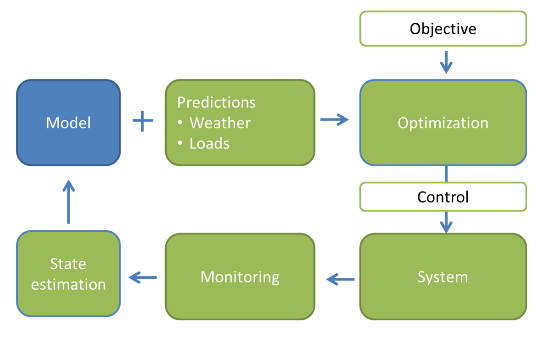
Fig. 11.1 MPC architecture.

The MPC runs online repeatedly through the loop presented in Fig. 11.1. With a system model and predictions of weather and internal load, an optimal control problem is solved to find the control variables which minimize the objective function over the prediction horizon. Since neither the model nor the predictions are perfect, a feedback loop is implemented. The heating system water temperature and the zone air temperature measurements from the building monitoring system are used to correct erroneous predictions through a simple moving horizon state estimation algorithm, which updates the states of the model based on measurements. With the new model state the next optimization loop starts.

The optimal control problem in the MPC is solved using JModelica [AAG+10], based on a toolbox written in Python to implement optimization problems using Modelica models. The reason for using Modelica and JModelica in the approach of MPC is twofold. First, the models implemented to represent the thermal behavior of the building and heating system are constructed in Modelica. The object-oriented implementation allowed constructing a library of low order resistance-capacitance models to represent the thermal system. A python toolbox implemented in JModelica allows for identification of model parameter values by solving an optimization problem that fits the model building temperature outputs to real measurements [DCMAH15]. Parameters of several model structures were identified, and from these, the best fitted model was selected. Secondly, JModelica was used to set up the optimal control problem. Since JModelica uses gradient-based methods for solving an optimal control problem, the equation based Modelica models are particularly well-suited as they allow symbolic differentiation and analysis of the model structure.

11.4.1.2. MPC for Chiller Plants

This case study presents the implementation of MPC for a chiller plant in order to improve the operating efficiency of the plant. To facilitate the implementation of the MPC, a software environment was developed consisting of three modules as shown in Fig. 11.2: Dynamic Optimization, Pre-processing and Post-processing. As the core of the framework, the Dynamic Optimization module is composed of an optimization engine and a system model. Raw measured data from the plant is processed in the Pre-processing module, which cleans it for input into the Dynamic Optimization module. The optimization results are then processed in the Post-processing module. Modelica is used to build the system model for the entire chiller plant (the primary chilled water loop and the condenser water loop).

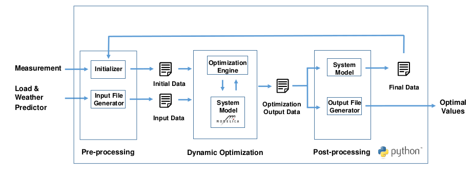
Fig. 11.2 MPC for chiller plants workflow.

In Fig. 11.2, the Dynamic Optimization module is designed to perform the optimization of the control inputs for the chiller plant. The objective function of the optimization is the energy consumption of the chiller plant during the optimization period. The optimized control inputs are the condenser water set point and the thresholds for chiller staging. The input variables for the optimization are the cooling load, the outdoor wet bulb temperature and the state of the controller. The Pre-processing module contains two components: Initializer and Input File Generator. The Initializer generates the Initial Data based on the Final Data from the previous optimization period. The Input File Generator converts the raw data, such as cooling load and weather data, into the Input Data, which can be directly read by the System Model. In the Post-processing module, the System Model reads the Optimization Output Data and generates the Final Data, which is then used for the next optimization period. The Final Data module includes the state vector. In addition, a component called Output File Generator processes the raw data in the Optimization Output Data and exports the data for later use, such as for plotting the results and generating the control signals.

For our experiments, we used the Dymola simulation environment. Dymola, as other Modelica environments, allow easy reseting of state variables which is needed when solving the optimal control problem, and when advancing time during the MPC algorithm. Of further benefit was the adaptive time step solver, which adjusted the time step automatically, selecting smaller time steps in times when the system changes rapidly. This lead to fast simulation time, while properly representing the dynamics of the process.

11.4.1.3. MPC for Energy Control of Underground Public Spaces

This case study describes the MPC implementation on the forced ventilation system in the Passeig De Gracia Metro Station in Barcelona (Spain). Given the complexity of the environment and the safety requirements specified, an MPC engineering framework was designed to minimize the impact of the system development on the station operation. Within this framework, Modelica was used to develop the whole building metro station model, including thermal and fluid dynamics, ventilation and lighting systems, and train and passenger flows. This system model was then used as an emulator to train a Bayesian Network that was used inside the MPC. Despite the size of the resulting model, amounting to about 77,000 unknowns, the adopted Modelica development environment, Dymola, still provided manageable simulation times with respect to the overall MPC engineering requirements.

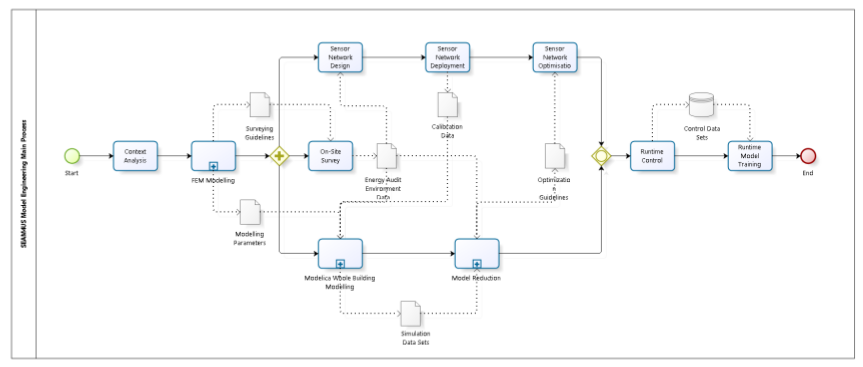
Fig. 11.3 MPC for energy control of underground public spaces workflow.

The MPC engineering workflow is depicted in Fig. 11.3. Context Analysis was aimed at surveying the site geometry, the plants technology and at assessing the original design. The characterization of the outdoor environment was accomplished through Finite Element modeling (FEM). It aimed at establishing the boundary conditions that influence the indoor dynamics. FEM was used to develop a preliminary model of the indoor environment as well, which informed a preliminary sensor network design. At this point, three tasks were started concurrently: on-site survey, the preliminary sensor network design and the development of the Modelica multi-physics station model. Despite the FEM modeling phase providing a number of insights regarding the behavior of the environment airflow and pollutants under different environmental conditions, it was limited to steady state analysis because of the size of the environment. This strongly limited its applicability to the development of complex MPC algorithms in the following phases, where optimality is achieved through accurate management of the transitory conditions. To this aim, Modelica provided a good compromise between expressiveness and computational efficiency. It endowed the abstraction and modularization that are required to manage the modeling complexity of such large domains. Knowledge encapsulation, topological interconnection, hierarchical modeling, and object orientation, as well as the availability of validated libraries granted operational effectiveness, and, at the same time, reduced the development effort. As soon as the first set of the monitoring data was available, the Modelica model was calibrated according to ASHRAE guidelines [ASH02]. This was a complex task and the computational stability and efficiency of the Modelica solvers were major factors in the success of this phase. Once calibrated, the Modelica station model was used to generate the data-set to train the Bayesian Network that was embedded in the deployed MPC loop and to fine tune the algorithms of the MPC systems without affecting the real station (Model Reduction). The flexibility of the Modelica environment was a major successful factor in this stage. The large station model was embedded as an FMU component in the MATLAB environment, and allowed for the development of optimal control algorithms in an emulated environment, without affecting the real station at all.

In this case study, Modelica proved effective as a fundamental part of a larger MPC engineering process. Modelica allows for the development of multi-physics domains made of thousands of components and evolving in a mixed continuous-discrete time model. Modelica is also an efficient language, as the solver speeds are adequate and the possibility of exporting FMUs opens possibilities of system integration. From an engineering perspective, the major limitations were associated with lack of a native support for model calibration, for which we used sensitivity and cluster analysis.

11.4.2. Fault Detection and Diagnosis

In building applications, the implementation of fault detection and diagnosis systems is usually programmed by experts for each specific plant, exploiting knowledge about the structure of the plant and the behavior of its components during correct and, if necessary, faulty conditions. These implementations, traditionally called expert systems, are typically structured as a set of rules that link potential symptoms and the faults possibly causing them, and an algorithm that applies the rules to given observations about the behavior of the system. The problem with this approach is not so much a technical one, but lies in the inevitably high efforts required to adapt or re-write the diagnostic program for a new plant or to reflect changes in an existing plant. The code (or the set of rules) has to be inspected in order to determine which part still applies and which must be modified or newly produced. The reason why these, often prohibitive, efforts are inevitable is that such programs capture the application of expert knowledge to a specific plant and, hence, leave both the structure of the plant and the knowledge about the physics of its components implicit in the code. A further drawback is that the set of rules is limited to symptoms and faults that have been experienced previously [Ste15].

Model-based fault detection and diagnosis overcomes these limitations by using models that provide an explicit representation of the knowledge about the components and the information about the plant structure, which determines how the components interact with each other. Based on a library of generic component models and the representation of the HVAC system topology, a system model (possibly covering both the nominal and faulty behaviors) can be obtained. The context-free component models allow for their re-use, the automated generation of system models, and, hence, cost-effective creation of new applications and easy adaptation to variants and modifications [Ste15]. The following examples demonstrate these benefits of using Modelica for FDD.

11.4.2.1. FDD for District Cooling Systems

The goal of this case study was to provide FDD and fault identification for a chilled water plant, including the increase in energy use or operational costs due to the fault. This data is provided to the operator in order to prioritize the urgency of correcting a fault. The project was conducted at the US Naval Academy in Annapolis (MD), which has a district cooling system with two plants that serve 20 buildings.

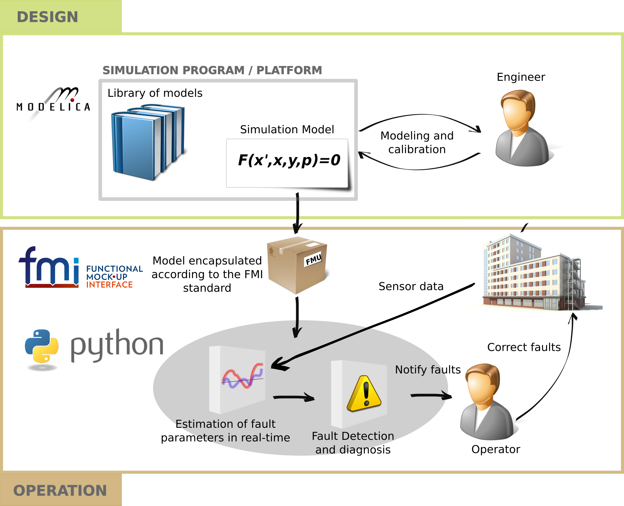
Fig. 11.4 Model-based fault detection using state estimation techniques compliant with the FMI standard.

Fig. 11.4 visualizes the approach used to implement the fault detection algorithm in the district cooling plant. The FDD algorithm is based on a state and parameter estimation algorithm that uses an Unscented Kalman Filter [BSG+14]. This requires repeated simulation of the model, subject to different parameters, initial states and input trajectories. The cooling plant and its components have been modeled using the Modelica Buildings library [WZNP14] and calibrated to measured data. The models were exported as an FMU for co-simulation and used during the operation of the plant within the FDD module, for representing the expected operation, and for computing the differences in energy and cost between faulty and correct operation. Python was used for the workflow automation, which consists of reading measured data from a data base, executing the state and parameter identification, which in turn executes the FMU for different inputs, initial states and parameters, and writing the results to a database for display to the operator in a web-based GUI. Fig. 11.5 shows parts of the GUI with monitored and estimated Coefficient of Performance (COP) of the chiller. The results of the state and parameter estimation algorithm are compared to the COP of the calibrated model. One of the advantages of this approach is that it provides a statistical description of the performance, and hence it allows to set fault thresholds based on a probability.

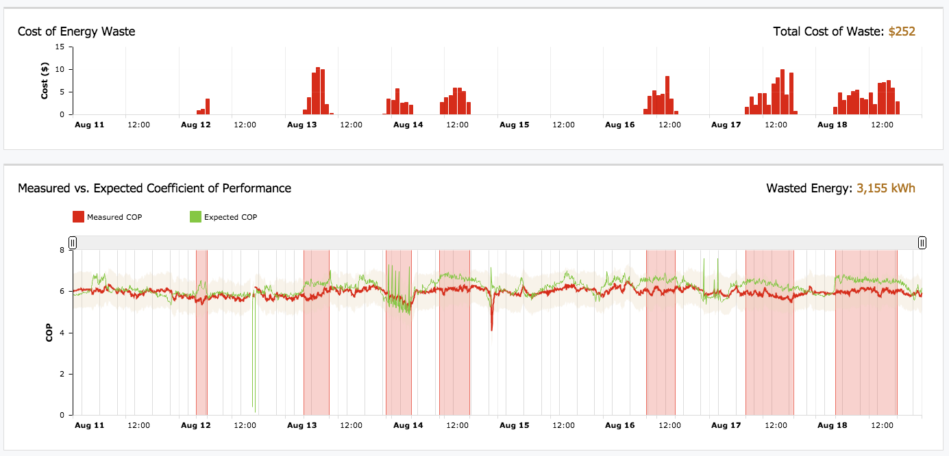
Fig. 11.5 Outputs of the fault identification algorithm, with costs caused by the fault (top graph) and comparison between measured and expected COP (bottom graph). The red rectangles are time intervals that have been identified as faulty periods in which the performance of the chiller was outside the tolerance.

Using Modelica allowed reusing a variety of component models from the Modelica Buildings library to build subsystem models of the chilled water plant, such as for the chillers and the cooling towers, which were then calibrated with measured data. After the calibration, these models were exported as FMUs in order to provide a model for the FDD algorithm. The use of FMUs has advantages in terms of compatibility and functionality. First, as FMI is a vendor-independent application programming interface for simulators, it allows the use of models authored by various modeling environments, thereby making the FDD framework independent of the model authoring tool. Second, the use of FMU allows to easily set values for the states, parameters and inputs for the repetitive simulations required by the FDD algorithm, as well as storing of final states for reuse as initial states for a new simulation.

11.4.2.2. FDD for Air Handling Units Components Using Qualitative Approaches

In contrast to quantitative models, qualitative models describe the behavior of a system only roughly. Instead of numerical values, qualitative models can deal with a symbolic representation of the system inputs, outputs and states, i.e. they can be represented by arguments like “high” or “low”

The process shown in Fig. 11.6 is a dynamic discrete-time, continuous-variable system whose qualitative behavior is described by a quantized system.

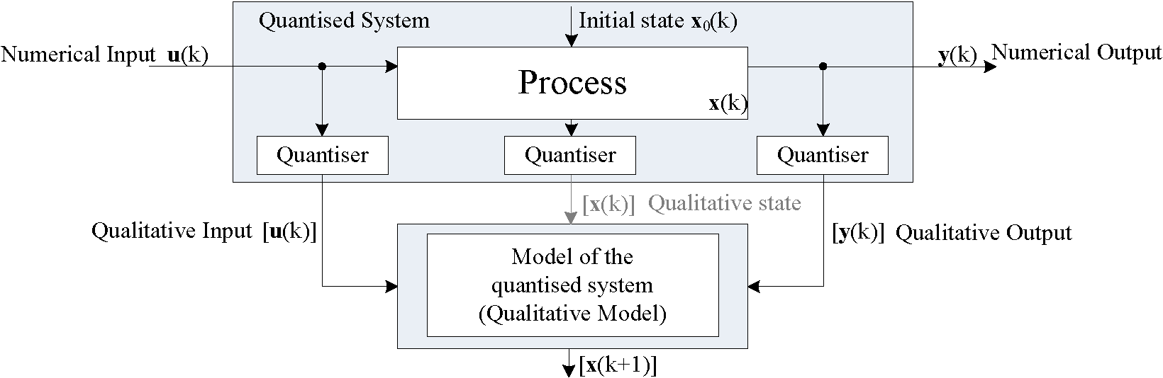
Fig. 11.6 Quantized System [S03].

We will now describe the qualitative approach that uses a stochastic automaton (SA) as the qualitative model. The qualitative model describes the qualitative behavior of the quantized system (see Fig. 11.6). Important work in this field has, e.g., been done by [Lun94]. Because the complexity of the so-called behavior tensor which stores the conditional probabilities of the state transitions of the automaton increases rapidly with a rising number of inputs, outputs and state signals, solutions for reducing the computational efforts and storage amounts are required. As shown in [MKLR15], the complexity of the behavior tensor of the SA can be reduced by exploiting the underlying tensor structure of the behavior relation. Therefore, a non-negative canonical polyadic (CP) tensor decomposition can be used to make qualitative models applicable to large discrete-time systems. Usually, qualitative models can be generated by an abstraction from a quantitative model or by stochastic qualitative identification. In our application, we will focus on the latter which has been developed by [Lic98]. The stochastic qualitative identification allows the generation of a qualitative model directly from measurement data or from simulation data. For both cases, for Fault Detection (FD) nominal data of the faultless system behavior is needed. Fault Detection and Diagnosis (FDD) requires also fault models or faulty measurement data. [LS96] used a qualitative observer for fault detection and diagnosis. Qualitative observation means the prediction of the possible system states at discrete time \(k+1\) based on the measured input and output combination at time \(k\). In general, the qualitative observer is the qualitative equivalent of e.g. the Luenberger observer known from continuous-time systems. The algorithm yields for each time step a probability vector describing the possible behavior of the system states for a given input.

If the probability vector contains only zeros, the measured input-output combination is inconsistent with the qualitative model and a fault can be structurally detected, [Lic98]. For demonstrating FD with qualitative models, different faults have been simulated with the Modelica fault triggering library, developed by the German Aerospace Center (DLR), [vdL14]. In the following, an application example of a heat exchanger of a HVAC&R system shows the applicability of the qualitative modeling approach.

We will now present an example. The considered system is a Heat Exchanger (HX) that cools air. It has been simulated with Modelica for the input signals shown in Fig. 11.7 for nominal and faulty conditions.

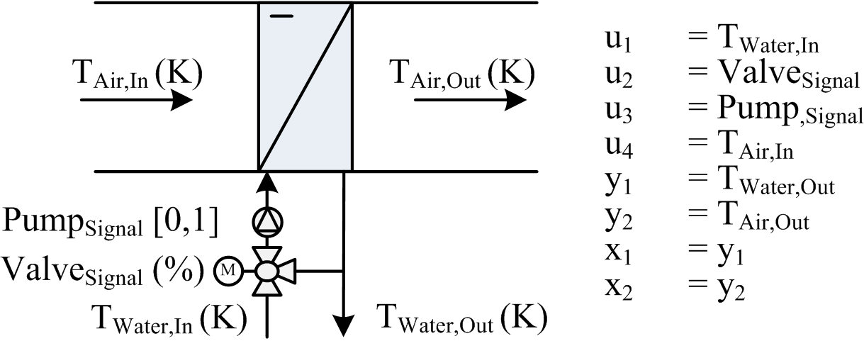
Fig. 11.7 Generic HX scheme.

The simulated fault describes a malfunction of the pump that leads to the problem of a fully opened valve, because the controller tries to track the set point of the air outlet temperature. Fig. 11.8 shows the faulty behavior during the time interval \(2420 \le t \le 2708\). As the figure shows, the air outlet temperature of the HX equals the air inlet temperature because no water circulates.

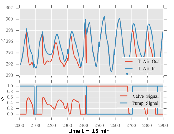
Fig. 11.8 Simulation Data.

Next, the qualitative model was trained using the nominal behavior of the HX as produced by the simulation model. Fig. 11.9 illustrates the qualitative state trajectory of the state variable \(T_{air, out}\) for a selected time range.

The state trajectory computed by the qualitative observation algorithm and it shows the probability distribution of the state signal for each discrete time step k. The different grey shades of the bars denote the probabilities. In the example, the state signal \(T_{air, out}\) was quantized into five intervals that can be seen by the horizontal separation of the black and grey bars.

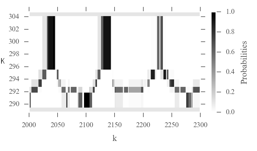
Fig. 11.9 Qualitative state trajectory of the air outlet temperature \(T_{air, out}\) (nominal condition).

Fig. 11.10 shows the qualitative state trajectory for the faulty condition. During the faulty operation, the measured input-output pair is inconsistent with the qualitative model, leading to components of the probability vector being close to zero. This is visualized by the white space in the figure for \(2420 \le k \le 2708\).

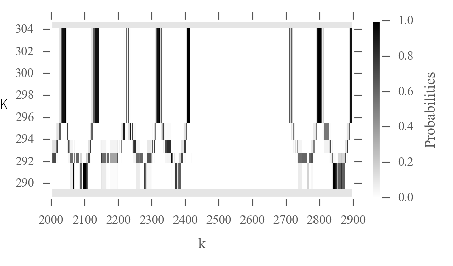
Fig. 11.10 Qualitative state trajectory of the air outlet temperature \(T_{air, out}\) (faulty condition).

For a better visualization, Fig. 11.11 displays 1 for non-faulty conditions and 0 for faulty conditions.

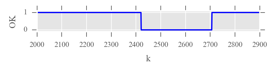
Fig. 11.11 Probability of the air outlet temperature x_2 (faulty condition).

While this example shows how fault detection with qualitative models can be realized, fault diagnosis is also possible. To achieve this, a set of qualitative models, where each model is trained with a different faulty condition has to be generated. Note that even for this simple example, the behavior relation of the SA contains over \(3.9 \cdot 10^6\) values, leading to a significant calculations for each discrete time step \(k\). For building automation systems (BAS), such high computing demands may not be possible. We therefore used a CP-decomposition, which reduced the size of the behavior relation by a factor of \(3200\) from \(3.9 \dot 10^6\) to \(1200\). This met the computing capabilities of the BAS for real-time application.

We will now turn the discussion to another case study. This case study demonstrates the use of Modelica to support a qualitative model-based fault detection and diagnosis approach based on first-order logic and a generic diagnosis algorithms. Model-based diagnosis is based on an explicit representation of the knowledge about the components and the information about the plant structure, which determines how the components interact with each other. Based on a Modelica library of generic component models representing first-principles of energy and mass transfer between components of the AHU and the representation of the AHU topology, a system model, possibly covering both the nominal and faulty behaviors, can be obtained. This model is then used by a generic diagnosis algorithm, which is neither plant- nor domain-specific. The diagnosis models used in qualitative model-based diagnosis are obtained by using the Modelica model to capture acceptable deviations of variables from their respective nominal behavior. Instead of using a stochastic automata, this method uses an inferencing system based on first-order logics to generate the diagnosis.

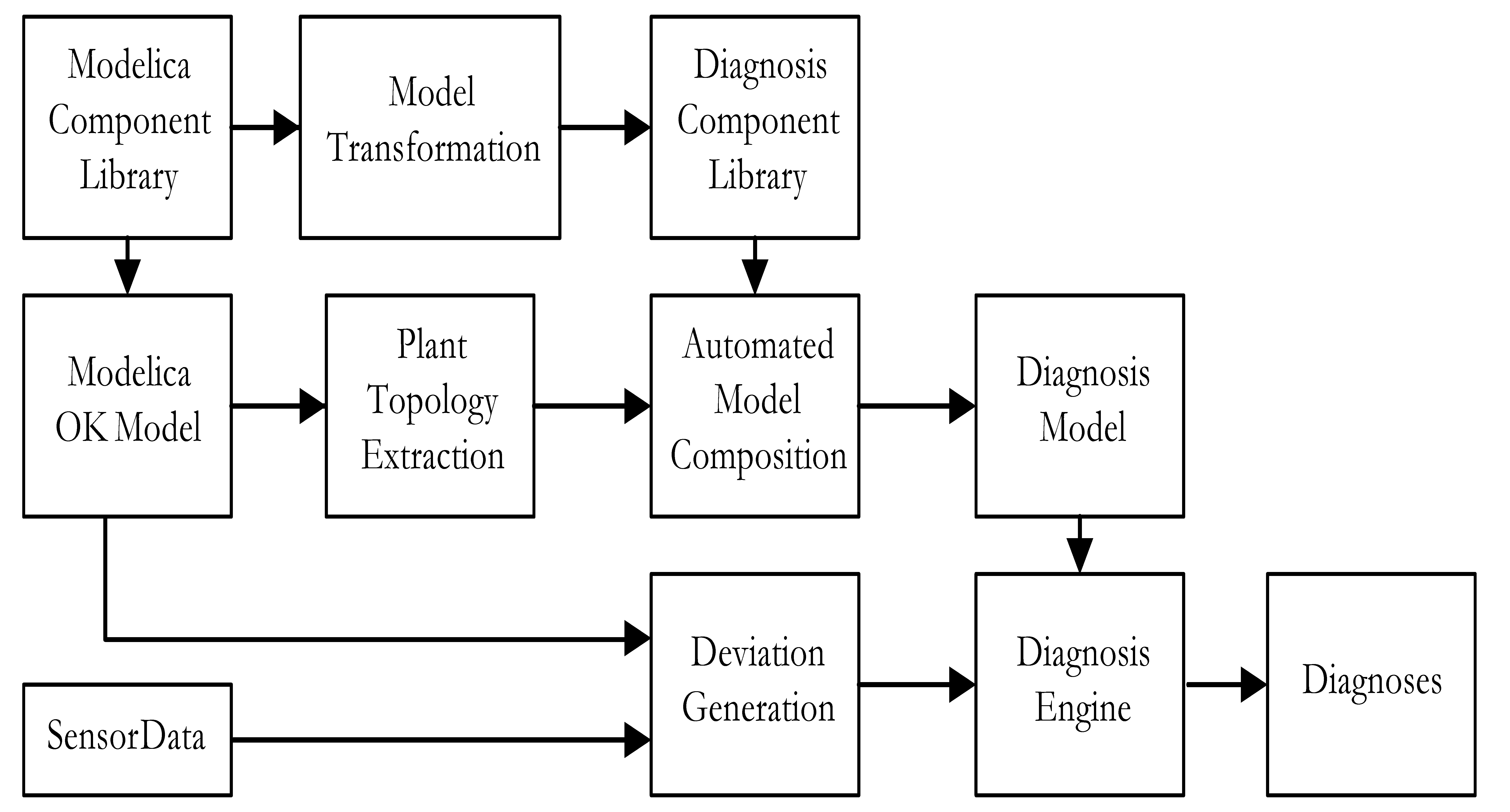
Fig. 11.12 Fault Detection of Air Handling Unit Components in a Qualitative Approach Workflow.

In Fig. 11.12, a complete workflow and system modules are presented that are required to build a diagnostic solution for a class of plants, such as HVAC systems, and to deploy and run it for a single plant. This process is referred to as qualitative model-based diagnosis. Here, we give an overview of the steps and modules. The steps are described in detail in [SPF+14] and are summarized as follows:

• Producing the general solution (top row) involves:

• The production of a library of Modelica models of the components (e.g. first principle models) [FSTK13] and
• its transformation into a qualitative diagnostic model library.

• Producing an application system (middle-row), based on the general solution, which requires:

• The configuration and calibration of the Modelica models of the correct behavior [FSK15], and
• the composition of the diagnostic model based on the diagnostic library and the topology of the plant, which can be extracted from the Modelica system model.

• For on-line diagnosis (bottom row):

• Computing the difference between the real data and the predictions generated by the Modelica model of the plant, and comparing the difference with given thresholds [SPF+14], and
• diagnosing the differences, using a runtime diagnosis engine such as Raz’r [OCCM14], which is an implementation of consistency-based diagnosis [MS96]. The output of the consistency-based diagnosis engine is a minimum set of combinations of component faults.

In this example, models were developed and applied to support model-based diagnosis. Use of Modelica led to a clear understanding of the underlying physical equation system since the equations within the component model and also on the level of the system model (connect equations) are clearly defined and can be easily reconstructed by the user of the model.

The main drawback of Modelica tools for this case study was the lack of native tools to interact with simulations during run-time. A python-Modelica interface needed to be developed. However, this need can nowadays be overcome by the use of FMI, for which Python interfaces are available.

11.4.2.3. FDD for Air Handling Unit Systems Using a Quantitative Approach

This case study focuses on the application of an open and replicable FDD method. The method consists of a combination of a Modelica model-based fault detection and a classifier-based diagnosis. It analyzes the monitored data on a real-time basis where a calibrated Modelica model evaluates the outputs from the outdoor conditions and the control signal and compares the estimation against the measurement to detect errors.

The method was used for component failure detection in an AHU, focusing on a prospective malfunction of the dampers, the heat recovery system and the fans. The AHU is part of a comprehensive test facility located on the KU Leuven Technology Ghent campus in Belgium. The facility is equipped with its own weather station measuring global solar irradiation, relative humidity, temperature, precipitation, wind speed and wind direction. A set of embedded sensors keep track of the AHU parameters such as the air volume flow, air temperature and relative humidity in the supply air and in the return air. The damper position signals are monitored as well. The monitored data are centralized and stored with a one minute frequency in a Soft-PLC based monitoring system where the BMS and the FDD algorithm is integrated on the same industry PC hardware.

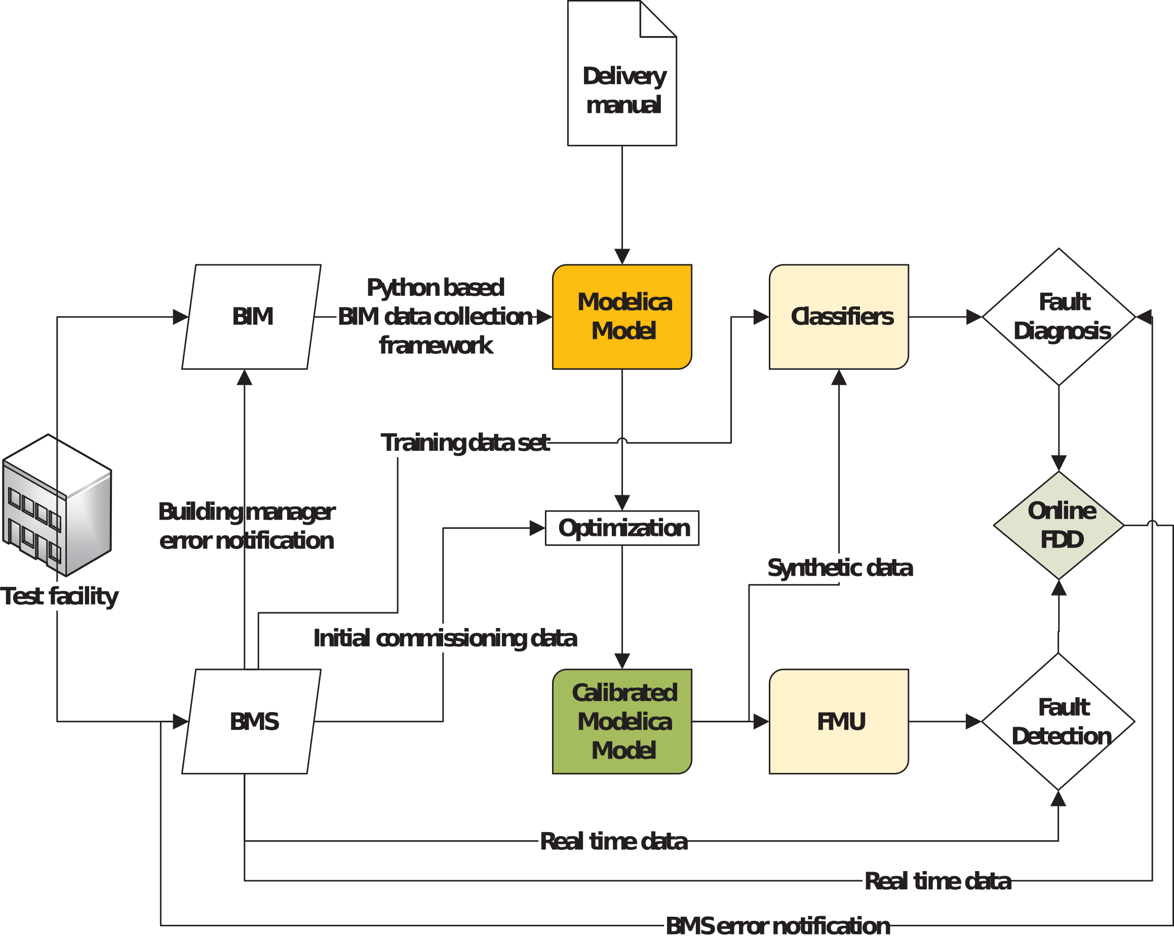
Fig. 11.13 Fault Detection of Air Handling Unit Systems in a Quantitative Approach Workflow.

As depicted in Fig. 11.13, a semi-automated BIM based process has been utilized to generate the Modelica model used for fault detection. It relies on a Python framework to extract and convert BIM data into a Modelica component compatible format. In this context, the BIM-based modeling approach is facilitated by the component-oriented feature of Modelica, which in turn allows an easy mapping between BIM objects and Modelica components. Data from the building delivery manual are used as input for the remaining parameter values not available in the BIM. An optimization-based calibration process is used to calibrate the Modelica model where a data set obtained throughout the initial commissioning process and assumed as fault free is utilized.

The Modelica model is exported as an FMU to be integrated into the BMS for a near-real time estimation of the outputs (e.g. supply air temperature). A discrepancy between the model estimation and the measurements superior to a predefined threshold is a sign of a likely issue on the system. To diagnose the error cause, the classifiers estimate the set of control signals which could provide the current output value as outcome. The cause of an error is isolated in a component if a discrepancy between the estimated and the actual control signal within this specific component is detected. In addition to the fault-free initial commissioning data, the classifiers are trained using synthetic data which represent several operating scenarios generated from the calibrated Modelica model.

An error notification is sent to the BMS if the algorithm detects the fault and its root cause is determined. An error notification is sent to the building manager if the occurrence of the error spans over a predefined period of time (e.g. 2 days). A BIM based error notification has been developed where the error location is pinpointed within the virtual representation of the building.

In this project, the use of Modelica was motivated by its ability to model the dynamic behavior of the components of the AHU. In addition, as an open language and considering the availability of open-source and validated libraries dedicated to buildings, Modelica fits well with developing an open FDD method.

11.4.3. Hardware in the Loop

Lastly, this section describes a hardware in the loop system. In this study, the Modelica Buildings library [WZNP14] is utilized to model an HVAC system that was used in a HIL setup to test the performance of closed loop control algorithms. During this project, the interface used to run Dymola models on the dSpace HIL simulator was still in development and not yet sufficiently reliable for utilization in this project. This was circumvented by importing the Dymola-generated code for the model in Simulink, and then using Simulink’s code generation functionality.

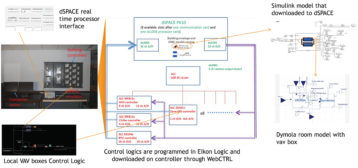
Fig. 11.14 Hardware in the loop workflow.

The pieces of equipment chosen to complete the loop in this study include a dSpace processor to execute models and a set of programmable VAV terminal controllers from Automated Logic Corporation (ALC). Additionally, digital-to-analog (D/A) and analog-to-digital (A/D) boards are used to establish communications between the dSpace and the controllers.

The model workflow shown in Fig. 11.14 mimics a room served by a VAV box with a reheat valve and a damper. This study focuses only on sensible heat transfer in buildings. Therefore, there is no humidity control and the air is assumed to be dry air. An AHU provides simple dry air at a prescribed temperature and sufficient pressure to overcome losses due to the damper and heat exchanger. The air is given a nominal flow rate, which serves as the flow rate of air with the damper fully open. From the AHU, the supply air flows through a heat exchanger block (i.e., reheat coil) with a constant effectiveness. Reheat is provided using a water-to-air heating coil, controlled by a linear two-way valve. Finally, the VAV damper is modeled using an exponential damper module from the Modelica Buildings library. The nominal supply airflow rate is set inside this module, and varies exponentially down to zero as the damper is closed. External signals are used to control both valve position on the reheat water loop and supply air damper position, as these signals will be received from the ALC controllers in the HIL simulation through an A/D board. Ideal flow and temperature sensors are placed throughout the model to monitor properties and ensure correct performance. Such sensor information was sent to ALC controllers through a D/A board. Finally, parameters that are not yet defined are set as inputs to the system. These will be declared later in Simulink, allowing them to be changed during real-time testing.

The room model in Fig. 11.14 describes a room using a thermal resistance-capacitance (RC) model and is modified from a RC model in the Modelica Annex60 library [WvTH13]. A capacitor for each surface represents thermal energy storage, followed by conduction and internal convection resistors. The ambient temperature is an input to the system, while the ground temperature is held at a constant value. Fluid ports allow the air from the VAV box to enter the room and return the air to an exit, maintaining the mass balance. Therefore, a fixed volume of air is maintained in the room at all times. There are a variety of assumptions made in this model, including the neglecting of infiltration and handling of outdoor convection as constant.

The combined thermal zone and VAV box model was downloaded to dSpace for the real-time execution. As previously mentioned, the model was first imported in Simulink for the code generation. This is possible using a Dymola-to-Simulink interface called DymolaBlock. This feature allows the model to be inserted into Simulink as a functional block whose outputs are calculated from defined inputs. In order to complete the loop, some parameters must be associated with D/A and A/D boards, and therefore either read from or sent to the real controllers. In this study, the room temperature is sent to the controller and the reheat valve position is returned for the heating model simulation. A dSpace blockset allows these communications to be defined in Simulink. Before building the model to code, a fixed step integrating method was selected. The model is then compiled to C code using Matlab, and the variable description files are downloaded onto dSpace for the real-time testing.

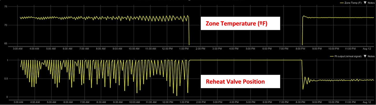
Fig. 11.15 Hardware in the loop results.

This HIL setup was used to test a conventional VAV box control called single maximum logic [TSPC12]. The outdoor air temperature was set to be very cold and the VAV box always stayed in the heating loop. Therefore only reheat valve position had to be controlled. The control was accomplished by using a PI block. Zone temperature and setpoint were compared to determine an appropriate reheat valve position, which was then sent to the Modelica model. The VAV box changed the model accordingly and solved for zone temperature at each time step, writing this value (sensor information) to the controllers to complete the loop. Both zone air temperature and reheat value position were trended and recorded in the BEMS (Fig. 11.15).

As can be seen in Fig. 11.15, the desired setpoint of the room was 72 Fahrenheit. The simulation was stopped around 1 pm and later resumed, with different PI loop tuning to illustrate the difference this can make. Before the re-tuning, wild fluctuations in the reheat valve were experienced. If this control were implemented in a real system, the constant opening and closing of the valve would lead to noise, wasted energy, discomfort, mechanical wear and eventually failure.

After a more optimal tuning was applied to the PI block, a classic underdamped oscillator curve can be seen. The reheat valve position ceases to undergo oscillatory changes, and finds a steady value to maintain room temperature at the setpoint. Reversals in signal can still be seen, but they are minimal compared to the prior tuning and are practically unavoidable.

During this study, sometimes compatibility issues have been encountered between the building code for dSpace and the Dymola-to-Simulink interface. This only occured with certain models, such as MixedAir from the Modelica Buildings library, and we have not yet located the root cause of these issues. These models work fine in Simulink but return a Simstruct Mex error during code generation. FMI usage should avoid such issues in future implementations.

11.5. Discussion and Conclusions

The use of Modelica to support the operation of building energy systems is promising as buildings involve multiple physical phenomena (e.g., heat transfer, fluid dynamics, electricity, etc.) and are complex in terms of their dynamics (e.g., coupling of continuous time physics with discrete time and discrete event control). Some clear advantages in the use of Modelica for supporting model use during operations include:

• The open source characteristic combined with the existence of several freely available Modelica libraries [BDCVR+12], [LTF+14], [NGHLR13], [WZNP14] allows for models to be modified and extended depending on the application requirements;
• Object-orientation not only enhances modularity and reusability of the models but also allows models to be developed following the physical system structure, which makes them easier to understand. The object-orientation enables extension and reuse of components and the use of standardized interfaces enables collaboration across physical domains and disparate developer groups.
• The Modelica object-oriented approach also allows for the development and the management of large and complex models. In such large-scale applications, the translators, the modeling language and environment are significantly stressed, and their robustness proved an enabling factor of the overall modeling process. This makes the Modelica toolchain well suited for handling highly complex models from the end user and the engineering perspective.
• The possibility to import and export Modelica models as Functional Mock-up Units (FMUs) enables the integration of models using a standardized, tool-independent API into existing FDD routines or the development of integral solutions that couple tools for data analysis, simulation, FDD and optimization in one single environment. An integral solution can be realized, for example, using the Building Controls Virtual Test Bed (BCVTB) [Wet11a] or JModelica with the Python module PyFMI [AAG+10].
• Modelica allows for a seamless use of the models developed in the design phase during the operational phase, for example, by exporting models as FMUs.

Finally, it is important to note that the advantages of Modelica can turn against the unexperienced developer. For example, because of the object-orientation employed in many libraries, it can be difficult to predict the depth to which a change in one component can have an effect in other components in the library. However, regression tests as are setup for the Modelica Annex60 library can detect such unintended side effects. In addition, the current capabilities of Modelica IDEs are still developing means to provide better debugging information. Also, training is highly recommended for novice users as the type of model verification and debugging done in equation-based languages differs from what users may be accustomed to when writing procedural code.