IEA EBC Annex 60

Annex60.Fluid.Examples.Performance

Package of examples that demonstrate computation speed performance

Information

This package contains examples that illustrate the Modelica conference paper by Jorissen et al. (2015) about speed optimization.

References

• Filip Jorissen, Michael Wetter and Lieve Helsen.
  Simulation speed analysis and improvements of Modelica models for building energy simulation.
  Submitted: 11th Modelica Conference. Paris, France. Sep. 2015.

Extends from Modelica.Icons.ExamplesPackage (Icon for packages containing runnable examples).

Package Content

Name	Description
Example1v1	Example 1 model without mixing volume
Example1v2	Example 1 model with mixing volume
Example2	Example 2 model with series pressure components
Example3	Example 3 model with mixed series/parallel pressure drop components
Example4	Example 4 model of simple condensing heat exchanger
Example5	Example 5 model of Modelica code that is inefficiently compiled into C-code
Example6	Example 6 model of Modelica code that is inefficiently compiled into C-code
Example7	Example 7 model of Modelica code that is more efficiently compiled into C-code
Example8	Common subexpression elimination example
BaseClasses

Annex60.Fluid.Examples.Performance.Example1v1

Example 1 model without mixing volume

Information

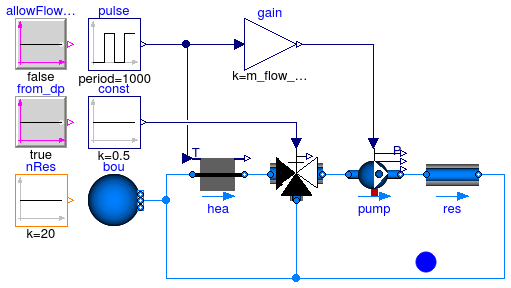
This model demonstrates the impact of the allowFlowReversal and from_dp parameters on the sizes of nonlinear algebraic loops. The user can change the parameter value in the respective BooleanConstant blocks and rerun the simulation to compare the performance. The results are also demonstrated below for nRes.k = 20, the number of parallel branches, which contain one pressure drop element each.

These results were generated using Dymola 2015FD01 64 bit on Ubuntu 14.04.

Default case:

AllowFlowReversal = true and from_dp = false

Sizes of nonlinear systems of equations: {6, 21, 46}

Sizes after manipulation of the nonlinear systems: {1, 19, 22}

Change 1:

AllowFlowReversal = false and from_dp = false

Sizes of nonlinear systems of equations: {6, 21}

Sizes after manipulation of the nonlinear systems: {1, 19}

Change 2:

AllowFlowReversal = false and from_dp = true

Sizes of nonlinear systems of equations: {6, 21}

Sizes after manipulation of the nonlinear systems: {1, 1}

These changes also have a significant impact on the computational speed.

Following script can be used in Dymola to compare the CPU times. For this script to work, make sure that Dymola stores at least 4 results.

cpuOld=OutputCPUtime;
evaluateOld=Evaluate;
OutputCPUtime:=true;
simulateModel("Annex60.Fluid.Examples.Performance.Example1v1(allowFlowReversal.k=true, from_dp.k=false)", stopTime=10000, numberOfIntervals=10, method="dassl", resultFile="Example1v1");
simulateModel("Annex60.Fluid.Examples.Performance.Example1v2(from_dp.k=true, allowFlowReversal.k=true)", stopTime=10000, numberOfIntervals=10, method="dassl", resultFile="Example1v2");
simulateModel("Annex60.Fluid.Examples.Performance.Example1v1(allowFlowReversal.k=false, from_dp.k=false)", stopTime=10000, numberOfIntervals=10, method="dassl", resultFile="Example1v1");
simulateModel("Annex60.Fluid.Examples.Performance.Example1v1(allowFlowReversal.k=false, from_dp.k=true)", stopTime=10000, numberOfIntervals=10, method="dassl", resultFile="Example1v1");
createPlot(id=1, position={15, 10, 592, 421}, range={0.0, 10000.0, -0.01, 0.35}, autoscale=false, grid=true);
plotExpression(apply(Example1v1[end-2].CPUtime), false, "Default case", 1);
plotExpression(apply(Example1v2[end].CPUtime), false, "Adding dummy states", 1);
plotExpression(apply(Example1v1[end-1].CPUtime), false, "allowFlowReversal=false", 1);
plotExpression(apply(Example1v1[end].CPUtime), false, "allowFlowReversal=false, from_dp=true", 1);
OutputCPUtime=cpuOld;
Evaluate=evaluateOld;

See Jorissen et al. (2015) for a discussion.

References

• Filip Jorissen, Michael Wetter and Lieve Helsen.
  Simulation speed analysis and improvements of Modelica models for building energy simulation.
  Submitted: 11th Modelica Conference. Paris, France. Sep. 2015.

Extends from Annex60.Fluid.Examples.Performance.BaseClasses.Example1 (Example 1 partial model).

Parameters

Modelica definition

Annex60.Fluid.Examples.Performance.Example1v2

Example 1 model with mixing volume

Information

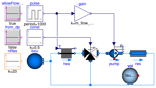
This example is an extension of Annex60.Fluid.Examples.Performance.Example1v1 and demonstrates the use of mixing volumes for decoupling the algebraic loop that solves for the enthalpy of the system.

Example1v1:

Sizes of nonlinear systems of equations: {6, 21, 46}

Sizes after manipulation of the nonlinear systems: {1, 19, 22}

Example1v2 using mixing volumes:

Sizes of nonlinear systems of equations: {6, 21, 4}

Sizes after manipulation of the nonlinear systems: {1, 19, 1}

See Jorissen et al. (2015) for a discussion.

References

• Filip Jorissen, Michael Wetter and Lieve Helsen.
  Simulation speed analysis and improvements of Modelica models for building energy simulation.
  Submitted: 11th Modelica Conference. Paris, France. Sep. 2015.

Extends from Annex60.Fluid.Examples.Performance.BaseClasses.Example1 (Example 1 partial model).

Parameters

Modelica definition

Annex60.Fluid.Examples.Performance.Example2

Example 2 model with series pressure components

Information

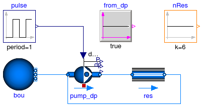
This example demonstrates that the use of the parameter from_dp can be important for reducing the size of algebraic loops in hydraulic circuits with many pressure drop components connected in series and a pump setting the pressure head.

If from_dp=true, we obtain:
Sizes of nonlinear systems of equations: {7}
Sizes after manipulation of the nonlinear systems: {5}
If from_dp=false, we obtain:
Sizes of nonlinear systems of equations: {7}
Sizes after manipulation of the nonlinear systems: {1}

This can have a large impact on computational speed.

Following script can be used in Dymola to compare the CPU times.

cpuOld=OutputCPUtime;
evaluateOld=Evaluate;
OutputCPUtime:=true;
simulateModel("Annex60.Fluid.Examples.Performance.Example2(from_dp.k=false)", stopTime=10000, numberOfIntervals=10, method="dassl", resultFile="Example2");
simulateModel("Annex60.Fluid.Examples.Performance.Example2(from_dp.k=true)", stopTime=10000, numberOfIntervals=10, method="dassl", resultFile="Example2");
createPlot(id=1, position={15, 10, 592, 421}, range={0.0, 10000.0, -0.01, 25}, autoscale=false, grid=true);
plotExpression(apply(Example2[end-1].CPUtime), false, "from_dp=false", 1);
plotExpression(apply(Example2[end].CPUtime), false, "from_dp=true", 1);
OutputCPUtime=cpuOld;
Evaluate=evaluateOld;


See Jorissen et al. (2015) for a discussion.

References

• Filip Jorissen, Michael Wetter and Lieve Helsen.
  Simulation speed analysis and improvements of Modelica models for building energy simulation.
  Submitted: 11th Modelica Conference. Paris, France. Sep. 2015.

Extends from Modelica.Icons.Example (Icon for runnable examples).

Parameters

Modelica definition

Annex60.Fluid.Examples.Performance.Example3

Example 3 model with mixed series/parallel pressure drop components

Information

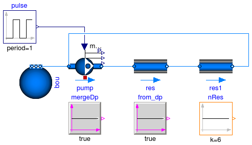
This example demonstrates the importance of merging pressure drop components that are connected in series, into one pressure drop component. Parameter mergeDp.k can be used to merge two components that are connected in series. Parameter from_dp also has an influence of the computational speed.

Following script can be used in Dymola to compare the CPU times. For this script to work, make sure that Dymola stores at least 4 results.

cpuOld=OutputCPUtime;
evaluateOld=Evaluate;
OutputCPUtime:=true;
simulateModel("Annex60.Fluid.Examples.Performance.Example3(from_dp.k=false, mergeDp.k=false, nRes.k=10)", stopTime=1000, numberOfIntervals=10, method="dassl", resultFile="Example3");
simulateModel("Annex60.Fluid.Examples.Performance.Example3(from_dp.k=false, mergeDp.k=true, nRes.k=10)", stopTime=1000, numberOfIntervals=10, method="dassl", resultFile="Example3");
simulateModel("Annex60.Fluid.Examples.Performance.Example3(from_dp.k=true, mergeDp.k=false, nRes.k=10)", stopTime=1000, numberOfIntervals=10, method="dassl", resultFile="Example3");
simulateModel("Annex60.Fluid.Examples.Performance.Example3(from_dp.k=true, mergeDp.k=true, nRes.k=10)", stopTime=1000, numberOfIntervals=10, method="dassl", resultFile="Example3");
createPlot(id=1, position={15, 10, 592, 421}, range={0.0, 1000.0, -0.01, 8}, autoscale=false, grid=true);
plotExpression(apply(Example3[end-3].CPUtime), false, "from_dp=false, mergeDp=false", 1);
plotExpression(apply(Example3[end-2].CPUtime), false, "from_dp=false, mergeDp=true", 1);
plotExpression(apply(Example3[end-1].CPUtime), false, "from_dp=true, mergeDp=false", 1);
plotExpression(apply(Example3[end].CPUtime), false, "from_dp=true, mergeDp=true", 1);
OutputCPUtime=cpuOld;
Evaluate=evaluateOld;

See Jorissen et al. (2015) for a discussion.

References

• Filip Jorissen, Michael Wetter and Lieve Helsen.
  Simulation speed analysis and improvements of Modelica models for building energy simulation.
  Submitted: 11th Modelica Conference. Paris, France. Sep. 2015.

Extends from Modelica.Icons.Example (Icon for runnable examples).

Parameters

Modelica definition

Annex60.Fluid.Examples.Performance.Example4

Example 4 model of simple condensing heat exchanger

Information

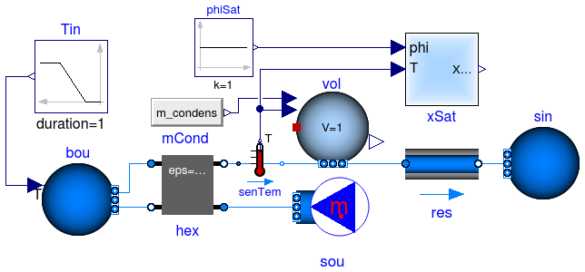
This example generates a non-linear algebraic loop that consists of 12 equations before manipulation. This loop can be decoupled and removed by changing the equation

port_a.m_flow + port_b.m_flow = -mWat_flow;

in Annex60.Fluid.Interfaces.StaticTwoPortConservationEquation to

port_a.m_flow + port_b.m_flow = 0;

See Jorissen et al. (2015) for a discussion.

References

• Filip Jorissen, Michael Wetter and Lieve Helsen.
  Simulation speed analysis and improvements of Modelica models for building energy simulation.
  Submitted: 11th Modelica Conference. Paris, France. Sep. 2015.

Extends from Modelica.Icons.Example (Icon for runnable examples).

Parameters

Modelica definition

Annex60.Fluid.Examples.Performance.Example5

Example 5 model of Modelica code that is inefficiently compiled into C-code

Information

This example illustrates the impact of Modelica code formulations on the C-code.

Compare the C-code in dsmodel.c when setting the parameter efficient to true or false and when adding annotation(Evaluate=true) to the parameter efficient.

This produces:

Efficient = false and Evaluate = false

helpvar[0] = sin(Time);
F_[0] = helpvar[0]*(IF DP_[0] THEN W_[0] ELSE DP_[1]+DP_[2]+DP_[3]);

Efficient = false and Evaluate = true

helpvar[0] = sin(Time);
F_[0] = helpvar[0]*(DP_[0]+DP_[1]+DP_[2]);

Efficient = true and Evaluate = true

helpvar[0] = sin(Time);
F_[0] = helpvar[0]*W_[1];

The last option requires much less operations to be performed and is therefore more efficient.

See Jorissen et al. (2015) for a discussion.

References

• Filip Jorissen, Michael Wetter and Lieve Helsen.
  Simulation speed analysis and improvements of Modelica models for building energy simulation.
  Submitted: 11th Modelica Conference. Paris, France. Sep. 2015.

Extends from Modelica.Icons.Example (Icon for runnable examples).

Parameters

Modelica definition

Annex60.Fluid.Examples.Performance.Example6

Example 6 model of Modelica code that is inefficiently compiled into C-code

Information

This example, together with Annex60.Fluid.Examples.Performance.Example7, illustrates the overhead generated by divisions by parameters. See Jorissen et al. (2015) for a complementary discussion.

Running the following commands allows comparing the CPU times of the two models, disregarding as much as possible the influence of the integrator:

simulateModel("Annex60.Fluid.Examples.PerformanceExamples.Example6", stopTime=100, numberOfIntervals=1, method="Rkfix4", fixedstepsize=0.001, resultFile="Example6");
simulateModel("Annex60.Fluid.Examples.PerformanceExamples.Example7", stopTime=100, numberOfIntervals=1, method="Rkfix4", fixedstepsize=0.001, resultFile="Example7");

Comparing the CPU times indicates a speed improvement of 56%. This difference almost disappears when adding annotation(Evaluate=true) to R and C.

In dsmodel.c we find:

DynamicsSection
W_[2] = divmacro(X_[0]-X_[1],"T[1]-T[2]",DP_[0],"R");
F_[0] = divmacro(W_[1]-W_[2],"Q_flow[1]-Q_flow[2]",DP_[1],"C");

This suggests that the parameter division needs to be handled during each function evaluation, probably causing the increased overhead.

The following command allows comparing the CPU times objectively.

simulateModel("Annex60.Fluid.Examples.Performance.Example6", stopTime=100, numberOfIntervals=1, method="Euler", fixedstepsize=0.001, resultFile="Example6");

See Jorissen et al. (2015) for a discussion.

References

• Filip Jorissen, Michael Wetter and Lieve Helsen.
  Simulation speed analysis and improvements of Modelica models for building energy simulation.
  Submitted: 11th Modelica Conference. Paris, France. Sep. 2015.

Extends from Modelica.Icons.Example (Icon for runnable examples).

Parameters

Modelica definition

Annex60.Fluid.Examples.Performance.Example7

Example 7 model of Modelica code that is more efficiently compiled into C-code

Information

See Annex60.Fluid.Examples.Performance.Example6 for the documentation.

Extends from Modelica.Icons.Example (Icon for runnable examples).

Parameters

Modelica definition

Annex60.Fluid.Examples.Performance.Example8

Common subexpression elimination example

Information

This is a very simple example demonstrating common subexpression elimination. The Dymola generated C-code of this model is:

W_[0] = sin(Time+1);
W_[1] = W_[0];

Hence, the sine and addition are evaluated once only, which is more efficient.

Extends from Modelica.Icons.Example (Icon for runnable examples).

Modelica definition